Introduction and Overview

This page offers a quick introduction to the theory and practice of meep_adjoint, beginning with a basic backgrounder on adjoint methods in general, then considering some representative design-optimization problems and outlining typical workflows for tackling in meep_adjoint. Adjoint experts will probably want to skim much of this before moving on to the detailed step-by-step tutorial, but are first encouraged at least to glance at our conventions for what constitute the :doc:`essential defining ingredients of optimization problems <OptProbIngredients_>`_.

Background: Automated design optimization and the adjoint method

Electromagnetic design optimization

A common task in electromagnetic engineering is to custom-tune the design of some component of a system—a waveguide taper, a power splitter, an input coupler, an antenna, etc.—to optimize the performance of the system as defined by some problem-specific metric. For our purposes, the performance metric will always be a physical quantity computed from frequency-domain electromagnetic fields—a power flux, an energy density, an eigenmode expansion coefficient, or perhaps some mathematical function of one or more such quantities—which we will denote \(f^\text{obj}\) or simply \(f\) and refer to as the objective function.

Meanwhile, the “design” entity that will be at our disposal to tweak and adjust in the service of optimizing \(f^\text{obj}\) will be just the spatially-varying scalar dielectric function \(\epsilon^\text{des}(\mathbf x)\) throughout some fixed subregion of the geometry (the design region \(\mathcal{V}^\text{des}\)). Of course, we will want to restrict consideration to designs that can actually be fabricated in the real world; at a minimum this means that the permittivity at each spatial point must satisfy the conditions imposed on physical materials by causality (which, for the simplest case of nondispersive dielectrics, are just that \(\epsilon\) be everywhere real-valued and \(\ge 1\)), but in some cases we might want to impose additional constraints—such as minimum linewidths—to reflect the limitations of practical fabrication techniques.

Thus, the problems we consider will be of the general schematic form

\[\text{ for } \mathbf{x} \in \mathcal{V}^\text{des}, \text{ find }\epsilon^\text{des}(\mathbf{x}) \text{ to optimize } f^\text{obj} \tag{1}\]

subject to the constraints that \(\epsilon^\text{des}\) be physical and (optionally) fabricatable.

First Examples: Holey waveguide and optical router

Here are two representative examples that we will use for illustrative purposes throughout this documentation (and for diagnostic purposes in the test suite).

First, the Holey Waveguide is a toy problem that fits the form of formulation: a simple section of waveguide, nearly pristine, but containing one region from which the dielectric material has been scooped out, leaving a hole:

In the presence of the hole, a wave entering the waveguide section from the left will be partially reflected, so that not all of the power it carries it will exit from the right. The design-optimization problem is to optimize the permittivity distribution in the hole region to maximize output power (for fixed input power). Obviously the correct answer is just to fill in the hole uniformly with the waveguide material, and the ability to figure this out is a simple, easy-to-debug test of the efficacy any optimization paradigm.

A less trivial example is the Cross Router, in which we envision 4 waveguides conjoined by a central hub region, whose design we will adjust to route signals from one port to another:

Examples

\[\epsilon^\text{design}(\mathbf x)\approx \sum_{d=1}^D \beta_d b_d(\mathbf x)\]

naively, this would give us uncountably many degrees of freedom and allow permittivity functions of arbitrarily rapid spatial variation, but such a design space would be both mathematically unwieldy and technologically unrealistic (in view of the finite lithographic linewidths and other constraints posed by real-world fabrication methods), whereupon in general we will approximate the design function as a finite expansion of the form

\[\epsilon^\text{design}(\mathbf x)\approx \sum_{d=1}^D \beta_d b_d(\mathbf x)\]

where \(\{b_d(\mathbf{x})\}, d=1,\cdots,D\) is some conveniently-chosen set of \(D\)

example in the meep_adjoint example gallery, the task is to design the central hub region to steer incoming power arriving via the West input waveguide port entirely to the North output waveguide port, ideally with zero leakage power emitted from the South and East

To formulate this problem mathematically, suppose we represent the unknown design function as an expansion in some convenient finite set of basis functions:

\[ \begin{align}\begin{aligned} \epsilon^\text{design}(\mathbf x)\approx \sum_{d=1}^D \beta_d b_d(\mathbf x)\\ Then, for given fixed values of the input power, operating frequency, and other parameters, the ia the **West** input waveguide port to the **North** output wav ple, in the :doc:`cross router <Examples/cross_router>` example in the :mod:`meep_adjoint` :doc:`example gallery <Examples/index>`, the task is to design the central hub region to steer incoming power arriving via the **West** input waveguide port entirely to the **North** output waveguide port, ideally with zero leakage power emitted from the **South** and **East**\\ To formulate this problem mathematically, suppose we represent the unknown design function as an expansion in some convenient finite set of basis functions:\end{aligned}\end{align} \]

\[ \begin{align}\begin{aligned} \epsilon^\text{design}(\mathbf x)\approx \sum_{d=1}^D \beta_d b_d(\mathbf x)\\ Then, for given fixed values of the input power, operating frequency, and other parameters, the ia the **West** input waveguide port to the **North** output wav ple, in the :doc:`cross router <Examples/cross_router>` example in the :mod:`meep_adjoint` :doc:`example gallery <Examples/index>`, the task is to design the central hub region to steer incoming power arriving via the **West** input waveguide port entirely to the **North** output waveguide port, ideally with zero leakage power emitted from the **South** and **East**\\ To formulate this problem mathematically, suppose we represent the unknown design function as an expansion in some convenient finite set of basis functions:\end{aligned}\end{align} \]

\[ \begin{align}\begin{aligned} \epsilon^\text{design}(\mathbf x)\approx \sum_{d=1}^D \beta_d b_d(\mathbf x)\\ Then, for given fixed values of the input power, operating frequency, and other parameters, the ia the **West** input waveguide port to the **North** output wav ple, in the :doc:`cross router <Examples/cross_router>` example in the :mod:`meep_adjoint` :doc:`example gallery <Examples/index>`, the task is to design the central hub region to steer incoming power arriving via the **West** input waveguide port entirely to the **North** output waveguide port, ideally with zero leakage power emitted from the **South** and **East**\\ To formulate this problem mathematically, suppose we represent the unknown design function as an expansion in some convenient finite set of basis functions:\end{aligned}\end{align} \]

\[ \begin{align}\begin{aligned} \epsilon^\text{design}(\mathbf x)\approx \sum_{d=1}^D \beta_d b_d(\mathbf x)\\ Then, for given fixed values of the input power, operating frequency, and other parameters, the ia the **West** input waveguide port to the **North** output wav ple, in the :doc:`cross router <Examples/cross_router>` example in the :mod:`meep_adjoint` :doc:`example gallery <Examples/index>`, the task is to design the central hub region to steer incoming power arriving via the **West** input waveguide port entirely to the **North** output waveguide port, ideally with zero leakage power emitted from the **South** and **East**\\ To formulate this problem mathematically, suppose we represent the unknown design function as an expansion in some convenient finite set of basis functions:\end{aligned}\end{align} \]

\[ \begin{align}\begin{aligned} \epsilon^\text{design}(\mathbf x)\approx \sum_{d=1}^D \beta_d b_d(\mathbf x)\\ Then, for given fixed values of the input power, operating frequency, and other parameters, the ia the **West** input waveguide port to the **North** output wav ple, in the :doc:`cross router <Examples/cross_router>` example in the :mod:`meep_adjoint` :doc:`example gallery <Examples/index>`, the task is to design the central hub region to steer incoming power arriving via the **West** input waveguide port entirely to the **North** output waveguide port, ideally with zero leakage power emitted from the **South** and **East**\\ To formulate this problem mathematically, suppose we represent the unknown design function as an expansion in some convenient finite set of basis functions:\end{aligned}\end{align} \]

\[ \begin{align}\begin{aligned} \epsilon^\text{design}(\mathbf x)\approx \sum_{d=1}^D \beta_d b_d(\mathbf x)\\ Then, for given fixed values of the input power, operating frequency, and other parameters, the ia the **West** input waveguide port to the **North** output wav ^\text{design}(\mathbf x)\approx \sum_{d=1}^D \beta_d b_d(\mathbf x)\\ Then, for given fixed values of the input power, operating frequency, and other parameters, the ia the **West** input waveguide port to the **North** output wav scalar basis functions defined for\end{aligned}\end{align} \]

\(\mathbf{x}\in\mathcal{V}^\text{design}\). This restricts the space of possible design functions to the span of the \(\{b_d\}\) and reduces our mathematical problem to finding values for the \(\{\beta_d\}\) coefficients that optimize the objective function—subject, of course, to appropriate physicality constraints on $epsilon$. If we restrict consideration to nondispersive media, the conditions for a physical permittivity are simply \(\text{Re }\epsilon\ge 1, \text{Im }\epsilon = 0\), and the mathematical formulation of our design challenge takes the form

(1)\[ \begin{align}\begin{aligned} \text{find } \boldsymbol{\beta} \in \mathbb{R}^D \text{ such that } f^\text{obj}(\boldsymbol{\beta}) = \text{optimum},\\ \text{subject to} \sum_{d=1}^D \beta_d b_d(\mathbf x) \ge 1, \,\,\,\, \forall \,\,\,\, \mathbf{x} \in \mathcal{V}^\text{design}\end{aligned}\end{align} \]

This is a $D$-dimensional optimization problem subject to linear inequality constraints.[#]_

We will shortly present a smorgasbord of examples; for now, perhaps a good one to have in mind is the [hole cloak ](#HoleCloak) discussed below, in which a chunk of material has been removed from an otherwise perfect waveguide section, ruining the otherwise perfectly unidirectional (no scattering or reflection) flow of power from a source at one end of the guide to a sink at the other; our task is to tweak the permittivity in an annular region surrounding the defect (the cloak) so as to restore as much as possible the reflectionless transfer of power across the waveguide—thus hiding or “cloaking” the presence of defect from external detection.

Now, for a given a candidate design \(\epsilon^{\text{trial}}(\mathbf{x})\), it’s clear that we can use meep—coremeep, that is, no fancy new packages required—to evaluate the objective function and assess the candidate’s performance: we simply (1) create a meep geometry with GeometricObjects for the waveguides and a Block with \(\epsilon\sup{trial}\) as a spatially-varying permittivity function in the design region, (2) add DFT cells to tabulate the frequency-domain Poynting flux entering and departing the cloak region, (3) timestep until the frequency-domain fields converge, then (4) use post-processing routines like ` get_fluxes() <GetFluxes>`_ or ` get_eigenmode_coefficients <EigenCoefficients>`_ to get the quantities needed to evaluate the objective function. This is a totally standard application of canonical meep functionality, and it has the effect of converting our engineering design problem into a pure numerical optimization problem: given a

Thus, for the cost of one full meep timestepping run we obtain the value of our objective function at one point in the parameter space of possible inputs.

…but function values alone aren’t enough for efficient optimization.

But now what do we do?! The difficulty is that the computation izinust described furnishes only the value of the objective function for a given input, not its derivatives with respect to the design variables—and thus yields zero insight into how we should tweak the design to improve performance. In simple cases we might hope to proceed on the basis of physical intuition, while for small problems with just a few parameters we might try our luck with a derivative-free optimization algorithm; however, both of these approaches will run out of steam long before we scale up to the full complexity of a practical problem with thousands of degrees of freedom. Alternatively, we could get approximate derivative information by brute-force finite-differencing—slightly tweaking one design variable, repeating the full timestepping run, and asking how the results changed—but proceeding this way to compute derivatives with respect to all \(D\) design variables would require fully \(D\) separate timestepping runs; for the problem sizes we have in mind, this would make calculating the objective-function gradient several thousand times more costly than calculating its value. So we face a dilemma: How can we obtain the derivative information necessary for effective optimization in a reasonable amount of time? This is where adjoints come to the rescue.

meep_adjoint is a tool for computing objective-function gradients.

The adjoint method of sensitivity analysis is a technique in which we exploit certain facts about the physics of a problem and the consequent mathematical structure—specifically, in this case, the linearity and reciprocity of Maxwell’s equations—to rearrange the calculation of derivatives in a way that yields an enormous speedup over the brute-force finite-difference approach. More specifically, after we have computed the objective-function value by doing the full meep timestepping run mentioned above—the “forward” run in adjoint-method parlance—we can magically compute its derivatives with respect to all design variables by doing just one additional timestepping run with a funny-looking choice of sources and outputs (the “adjoint” run). Thus, whereas gradient computation via finite-differencing is at least \(D\) times more expensive than computing the objective function value, with adjoints we get both value and gradient for roughly just twice the cost of the value alone. Such a bargain! At this modest cost, derivative-based optimization becomes entirely feasible.

Examples of optimization problems

Throughout the meep_adjoint documentation we will refer to a running collection of simple optimization problems to illustrate the mechanics of optimization, among which are the following; click the geometry images to view in higher resolution.

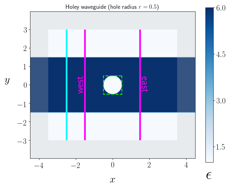
The Holey Waveguide

By way of warm-up, a useful toy version of an optimization problem is an otherwise pristine length of dielectric slab waveguide in which a careless technician has torn a circular hole of variable permittivity \(\epsilon\sup{hole}\).

> :bookmark:{.center} > > 

Incident power from an eigenmode source (cyan line in figure) travels leftward through the waveguide, but is partially reflected by the hole, resulting in less than 100% power the waveguide output (as may be characterized in meep by observing power flux and/or eigenmode expansion coefficients at the two flux monitors, labeled east and west). Our objective is to tweak the value of \(\epsilon\sup{hole}\) to maximize transmission as assessed by one of these metrics. The simplicity of this model makes it a useful initial warm-up and sanity check for making sure we know what we are doing in design optimization; for example, `in this worked example <AdjointVsFDTest_>`_ we use it to confirm the numerical accuracy of adjoint-based gradients computed by mp.adjoint

The Hole Cloak

We obtain a more challenging variant of the holey-waveguide problem be supposing that the material in the hole region is not a tunable design parameter—it is fixed at vacuum, say, or perfect metal—but that we are allowed to vary the permittivity in an annular region surrounding the hole in such a way as to mimic the effect of filling in the hole, i.e. of hiding or “cloaking” the hole as much as possible from external

detection.

> :bookmark:{.center} > > 

For the hole-cloak optimization, the objective function will most likely the same as that considered above—namely, to maximize the Poynting flux through the flux monitor labeled east (a quantity we label \(S\subs{east}\))

or perhaps to maximize the overlap coefficient

between the actual fields passing through monitor east and the fields of (say) the \(n\){P,M}_{n,text{east}}` with \(P,M\) standing for “plus and minus.”) On the other hand, the design space here is more complicated than for the simple hole, consisting of all possible scalar functions \(\epsilon(r,\theta)\) defined on the annular cloak region.

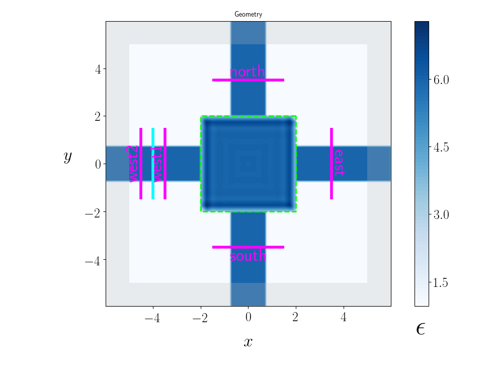
The cross-router

A different flavor of waveguide-optimization problem arises when we consider the routing of signals from given inputs to given destinations. One example is the cross-router, involving an intersection between :math:`x-`directed and :math:`y-`directed waveguides, with center region of variable permittivity that we may tweak to control the routing of power through it.

> :bookmark:{.center} > > 

Whereas in the previous examples there was more or less only one reasonable design objective one might realistically want to optimize, for a problem like this there are many possibilities. For example, given fixed input power supplied by an eigenmode source on the “western” branch (cyan line), we might be less interested in the absolute output power at any port and more concerned with achieving maximal equality of output power among the north, south, and east outputs, whereupon we might minimize an objective function of the form :math:``fsub{obj} =

Big( Ssub{north} - Ssub{south}Big)^2

+Big( Ssub{north} - Ssub{east}Big)^2

• Big( Ssub{east} - Ssub{south}Big)^2

:math:`` (or a similar functional form involving eigenmode coefficients). Alternatively, perhaps we don’t care what happens in the southern branch, but we really want the fields traveling past the north monitor to have twice as much overlap with the forward-traveling 3rd eigenmode of that waveguide as the east fields have with their backward-traveling 2nd eigenmode:

:math:`` fsub{obj} equiv Big( Psub{3,north} - 2Msub{2,east}Big)^2:math:``

The point is that the definition of an optimization problem involves not only a set of physical quantities (power fluxes, eigenmode coefficients, etc.) that we compute from meep calculations, but also a rule (the objective function \(f\)) for crunching those numbers in some specific way to define a single scalar figure of merit.

In mp.adjoint we use the collective term objective quantities for the power fluxes, eigenmode coefficients, and other physical quantities needed to compute the objective function. Similarly, the special geometric subregions of meep geometries with which objective quantities are associated—the cross-sectional flux planes of DFTFlux cells or field-energy boxes of DFTField cells—-are known as objective regions.

The `Example Gallery <ExampleGallery.md_>`_ includes a worked example of a full successful iterative optimization in which mp.adjoint begins with the design shown above and thoroughly rejiggers it over the course of 50 iterations to yield a device that efficiently routs power around a 90&degree; bend from the eigenmode source (cyan line above) to the ‘north’ output port.

The asymmetric splitter

A splitter seeks to divide incoming power from one source in some specific way among two or more destinations., We will consider an asymmetric splitter in which power arriving from a single incoming waveguide is to be routed into two outgoing waveguides by varying the design of the central coupler region:

> :bookmark:{.center} > > 

Defining elements of optimization problems

The examples above, distinct though they all are, the common set of ingredients required for a full specification of an optimization problem.

In brief,

for use in computing power fluxes, mode-expansion coefficients, and other frequency-domain

quantities used in characterizing device performance. Because these regions are used to evaluate

objective functions, we refer to them as objective regions.

• Design region: A specification of the region over which the material design is to be

  optimized, i.e. the region in which the permittivity is given by the design quantity \(\epsilon\sup{des}(\mathbf x)\). We refer to this as the design region \(\mathcal{V}\sup{des}\).

• Basis: Because the design variable \(\epsilon\sup{des}(\mathbf x)\)

  is a continuous function defined throughout a finite volume of space, technically it involves infinitely many degrees of freedom. To yield a finite-dimensional optimization problem, it is convenient to approximate \(\epsilon\sup{des}\) as a finite expansion in some convenient set of basis functions, i.e. :math:`` epsilon(mathbf x) equiv sum_{d=1}^N beta_d mathcal{b}_d(mathbf x),

  qquad mathbf xin mathcal{V}sup{des},

  :math:`` where \(\{\mathcal{b}_n(\mathbf x)\}\) is a set of \(D\) scalar-valued basis functions defined for \(\mathbf x\in\mathcal{V}\sup{des}\). The task of the optimizer then becomes to determine numerical values for the \(N\)-vector of coefficients \(\boldsymbol{\beta}=\{\beta_n\},n=1,\cdots,N.\)

  For adjoint optimization in meep, the basis set is chosen by the user, either from among a predefined collection of common basis sets, or as an arbitrary user-defined basis set specified by subclassing an abstract base class in mp.adjoint.

1

Technically, equation (1) appears to be imposing uncountably many constraints (one for each point \(\mathbf{x}\) in the design region) on our finite set of design variables; we will describe later how to extract a finite number of constraints for numerical optimization.

2

At present, maximization is the only supported optimization; if your objective is actually to minimize some quantity, just define the objective function with a minus sign. (Eventually some users might appreciate a --minimize option that would do this internally.)