

Computing T-Matrices of arbitrary objects with scuff-tmatrix

The well-known T-matrix method is a widely used technique for solving problems involving electromagnetic scattering from compact objects. In this method, the scattering properties of a compact body are encapsulated in its T-matrix, whose entries give the amplitudes of the outgoing spherical waves that arise from irradiating the object with a single regular spherical wave.

scuff-tmatrix is a specialized tool within the scuff-em code suite for computing the T-matrix of arbitrarily-shaped objects with arbitrary frequency-dependent material properties.

To compute the T-matrix of an object (or a collection of objects) using scuff-tmatrix, you will

1. create a geometry file describing the shapes and material properties of the scattering objects in your geometry;

2. run scuff-tmatrix with command-line options specifying the geometry, the maximum spherical-wave index $\ell^{\text{max}}$ of the spherical waves to consider (which determines the dimension of the computed T-matrix), and the frequency range over which to run computations.

You will get back

1. a text file listing the T-matrix elements $T_{\alpha\beta}(\omega)$, at all frequencies $\omega$ you requested, for all pairs of vector-spherical-wave indices $\alpha=\{\ell_\alpha,m_\alpha,P_\alpha\}, \beta=\{\ell_\beta,m_\beta,P_\beta\}$ satisfying $$1\le \ell \le \ell^{\text{max}}, \quad -\ell \le m \le +\ell, \quad P\in \{M,N\}$$

2. optionally, a binary .HDF5 file containing the T-matrix data together with simple scripts for importing the data into julia.

Table of Contents

• 1. scuff-tmatrix Command-Line Options
  • Options controlling the scattering geometry
  • Option describing the range of spherical-wave indices
• 2. scuff-tmatrix Output Files
  • 1. T-matrix data in text form
  • 2. T-matrix data in binary form
    • Ordering and indexing of spherical waves
• 3. scuff-tmatrix Examples
  • 4a. Dielectric and magnetic spheres
    • Analytical expressions for T-matrix elements
    • Geometry and mesh files
    • Frequency list
    • Run scuff-tmatrix
• 4. Reading T-Matrix data into julia

1. scuff-tmatrix Command-Line Options

The following table summarizes all command-line options currently available in scuff-tmatrix.

As is true for all programs in the scuff-em suite, command-line options may be specified in a text file catted to standard input; see here for an example of how this works.

Options controlling the scattering geometry

--geometry MyGeometry.scuffgeo

Specifies the geometry file describing the scattering geometry. This option is always mandatory.

Options specifying the frequencies considered

--Omega xx 

--OmegaFile MyFile

--Omega specifies an angular frequency at which to run computations, in units of $\omega_0 \equiv 3\times 10^{14}$ rad/sec ($=c/1 \mu$m).

The value specified for --Omega may be a complex number.

You may request computations at more than one frequency by using the --Omega option more than once, i.e. you may say

--Omega 1e-2 --Omega 1e-1 --Omega 1 --Omega 10

However, for more than a few frequencies it is more convenient to use the --OmegaFile option, which specifies a file containing an entire list of --Omega values, one per line; blank lines and comments (lines beginning with #) are skipped.

Option describing the range of spherical-wave indices

--lMax 3

Request calculation of T-matrix entries with spherical wave indices up to and including $\ell=\ell^{\text{max}}$ (and all $m$-values and polarizations). As described below, for a maximum $\ell$-value of $\ell^\text{max}$ the $T$-matrix has dimension $D\times D,$ where $D=2(\ell^{\text{max}}+1)^2 - 2$.

If you do not specify this option, the default value is lMax=3.

Options controlling output files

--FileBase MyFileBase

Sets the base file name for output files. T-matrix data in text format are written to FileBase.TMatrix. T-matrix data in binary (HDF5) format are written to FileBase_wXXXX.HDF5 where XXXX denotes the angular frequency.

If not specified, --FileBase defaults to the base filename of the .scuffgeo file.

--WriteHDF5Files 

This boolean flag requests that binary T-matrix data be written to HDF5 files. A separate HDF5 file is created for each frequency, with file name FileBase_wXXXX.HDF5 where XXXX denotes the angular frequency. T matrix data are written in the form of a real-valued matrix (data set) named T with dimension $D\times 2D$; for $d=0,1,\cdots,D-1,$ columns $2d$ and $2d+1$ give the real and imaginary parts of the $T$-matrix entry for column $d$. Here $D=2(\ell^{\text{max}}+1)^2 - 2$ is the total number of vector spherical waves with $1\le \ell \le \ell^{\text{max}}.$ (T-matrix rows and columns are indexed as shown in this table.)

Note that, in contrast to text-based output, binary data output is disabled by default; you must specify this option to enable binary data output.

2. scuff-tmatrix Output Files

1. T-matrix data in text form

scuff-tmatrix always writes T-matrix data to a text-based output file named FileBase.TMatrix, where FileBase is the value you gave for the --FileBase command-line parameter. (If you didn't set this option, FileBase defaults to MyGeometry where MyGeometry.scuffgeo was the name of the file you specified with the --geometry option.)

Each line of the text-based output file contains a single T-matrix element at a single frequency. The format of each line is this:

---

Omega A La Ma Pa B Lb Mb Pb real(T) imag (T)

---

The tuple(A,La,Ma,Pa) labels the spherical wave that constitutes the row index for the T-matrix entry. (Here (La,Ma)=$(\ell_\alpha,m_\alpha)$ are the usual spherical-wave indices, Pa=$P_\alpha \in[0,1]$ is a polarization index (0 or 1 for $\mathbf{M}$ and $\mathbf{N}$-type vector spherical waves respectively) and A=$\alpha$ is an integer in the range $[0,D-1]$ that uniquely indexes the spherical wave. (See the table below).

The tuple(B,Lb,Mb,Pb) labels the spherical wave that constitutes the column index for the T-matrix entry.

The final two entries on the line are the real and imaginary parts of the T-matrix entry for the given pair of spherical waves at the given frequency.

Physically, the T-matrix element with row index $\alpha$ and column index $\beta$ is the amplitude of the outgoing spherical wave with indices $\{\ell,m,P\}_\alpha$ that results from illuminating your object with a regular spherical wave with indices $\{\ell,m,P\}_\beta$.

See below for a simple shell script you can use to extract a particular T-matrix entry vs. frequency from the .TMatrix file.

Also see below for a julia code that you can use to import T-matrix data into a julia session.

2. T-matrix data in binary form

If you specify the --WriteHDF5Files command-line argument, then T-matrix data will be written in binary HDF5 format to files named FileBase_wXXXX.HDF5 where XXXX stands for the angular frequency $\omega$.

Ordering and indexing of spherical waves

For a fixed single value of $\ell\ge 1$ there are $=2(2\ell+1)$ spherical waves: $(2\ell+1)$ pairs of spherical-wave indices $(\ell,m)$ times 2 polarizations (\mathbf{M},\mathbf{N}). The total number of distinct spherical waves $(\ell,m,P)$ with $1\le \ell \le \ell^{\text{max}}$ is $D=2(\ell^{\text{max}}+1)^2 - 2$. This is the dimension of the $T$ matrix computed at each frequency. (Note that I exclude $\ell=0$ waves from my indexing scheme entirely.)

The rows and columns of the $T$-matrix are indexed by integers $(\alpha,\beta)$ running from $0$ to $D-1$. Spherical waves are ordered and indexed as follows:

$$\begin{array}{|c|c|}\hline \alpha & (\ell,m,P) \\\hline 0 & (1,-1,0) \\\hline 1 & (1,-1,1) \\\hline 2 & (1, 0,0) \\\hline 3 & (1, 0,1) \\\hline 4 & (1, 1,0) \\\hline 5 & (1, 1,1) \\\hline 6 & (2,-2,0) \\\hline \vdots & \vdots \\\hline 15 & (2,+2,1) \\\hline 16 & (3,-3,0) \\\hline \vdots & \vdots \\\hline \end{array}$$ The integer index $\alpha$ for a given triple $(\ell, m, P)$ may be computed according to $$\alpha = 2\Big[\ell(\ell+1) + m - 1\Big] + P.$$

3. scuff-tmatrix Examples

Here are some examples of calculations you can do with scuff-tmatrix. Input files and command-line runscripts for all these examples are included in the share/scuff-em/examples subdirectory of the scuff-em installation.

4a. Dielectric and magnetic spheres

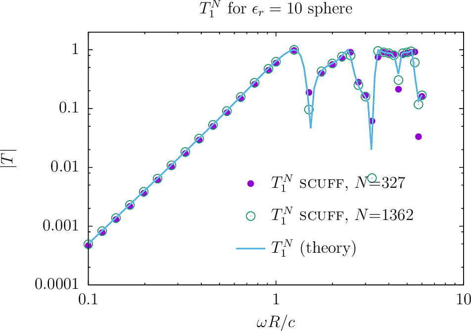
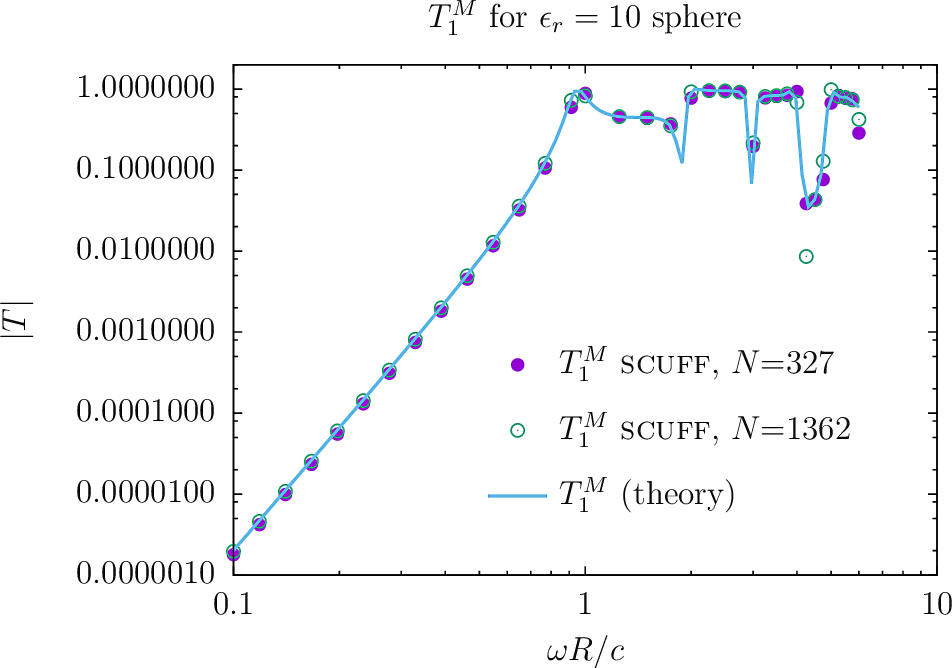
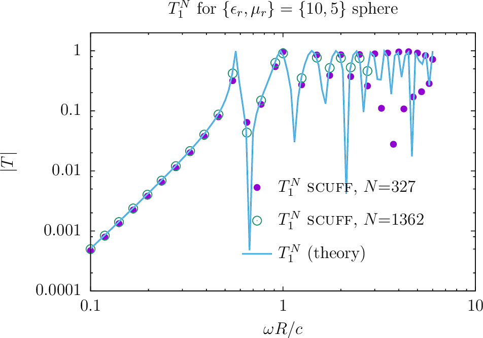
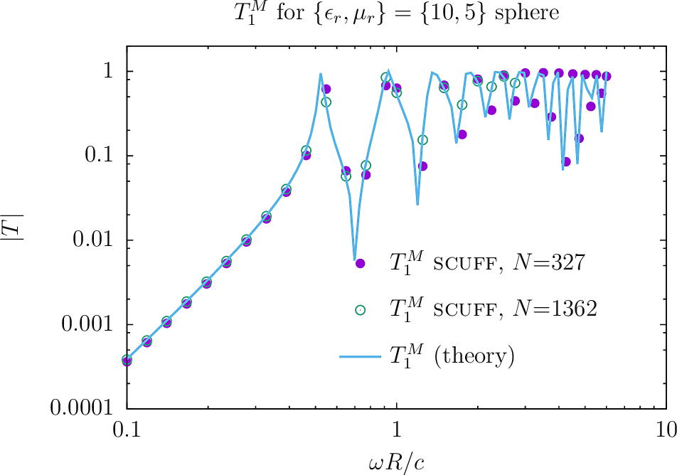
We start with the canonical textbook stalwart of scattering from a homogeneous sphere of uniform isotropic relative permittivity $\epsilon_r$ and relative permeability $\mu_r.$

Analytical expressions for T-matrix elements

This is an example (indeed, the only example) of a dielectric object whose T-matrix may be computed analytically, making it a useful benchmark for our numerical computation; the $T$-matrix is diagonal and independent of the $m$ spherical-wave index, with $\ell$-dependent elements

$$T_\ell^M = -\frac{ \mu_r j_\ell(na)\overline{j_\ell}(a) - j_\ell(a)\overline{j_\ell}(na) } { \mu_r j_\ell(na)\overline{h_\ell}(a) - h_\ell(a)\overline{j_\ell}(na) }$$ $$T_\ell^N = -\frac{ \epsilon j_\ell(na) \overline{j_\ell}(a) - j_\ell(a)\overline{j_\ell}(na) } { \epsilon j_\ell(na)\overline{h_\ell}(a) - h_\ell(a)\overline{j_\ell}(na) }$$ where $j_\ell$, $h_\ell$ are the usual spherical Bessel and Hankel functions and $$a=\frac{\omega R}{c}, \qquad n=\sqrt{\epsilon_r \mu_r}, \quad \overline{f(x)} \equiv f(x) + x\frac{d}{dx}f(x).$$

Geometry and mesh files

The first step is to create meshed surfaces representing spheres discretized with various resolutions, then write scuff-em geometry files describing spheres of various material properties. This process is described in detail here. In this case we will use two gmsh mesh files for a sphere of radius $R=1$:

• Sphere_327.msh, a moderate-resolution mesh with 327 internal triangle edges, and

• Sphere_1362.msh, a finer mesh with 1362 internal triangle edges.

For each meshing resolution I will create 3 .scuffgeo files describing spheres of different materials:

• perfect metal (PEC),

• homogeneous dielectric with $\epsilon_r=10$, and

• homogeneous dielectric/magnetic with $\epsilon_r=10, \mu_r=5$.

PECSphere_327.scuffgeo:

OBJECT Sphere
        MESHFILE Sphere_327.msh
ENDOBJECT

E10Sphere_327.scuffgeo:

OBJECT Sphere
        MESHFILE Sphere_327.msh
        MATERIAL CONST_EPS_10
ENDOBJECT

E10M5Sphere_327.scuffgeo:

OBJECT Sphere
        MESHFILE Sphere_327.msh
        MATERIAL CONST_EPS_10_MU_5
ENDOBJECT

Frequency list

We create a simple file called OmegaFile containing a list of angular frequencies (in units of $3\cdot 10^{14}$ rad/sec) at which to compute T-matrices:

0.10000000
0.11853758
....
6.00000000

Run scuff-tmatrix

And now we launch scuff-tmatrix:

% scuff-tmatrix --geometry E10Sphere_327.scuffgeo --omegafile OmegaFile --lmax 3

This produces the file E10Sphere_327.TMatrix, which contains one T-matrix entry per line, with a file header at the top to remind you which is which:

## scuff-tmatrix run on hikari (11/06/17::01:34:31)
## columns:
## 1 omega
## 2,3,4,5 (alpha, {L,M,P}_alpha)   (T-matrix row index)
## 6,7,8,9 ( beta, {L,M,P}_beta)    (T-matrix columnindex)
## 10, 11  real, imag T_{alpha, beta}
0.1  0 1 -1 +0   0 1 -1 +0  -1.34273817e-07 +3.62883443e-04
0.1  0 1 -1 +0   1 1 -1 +1  +1.13651828e-09 -1.05703395e-06
...
...
...
3.25  2 1 +0 0   9 2 -1 1  +8.56628506e-05 +2.48397970e-04
...
...
...

As an example, the lowest line above is interpreted as follows: At angular frequency $\omega=3.25 \times 3\cdot 10^{14}$ rad/sec, for the spherical-wave pair $(\alpha,\beta)=(2,9)$ [where $\alpha$ is a $\mathbf{M}$-type wave with $(\ell,m)=(1,0)$ and $\beta$ is an $\mathbf{N}$-type wave with $(\ell,m)=(2,-1)$, the $T$-matrix element is $$T_{2,9}(3.25) = 8.5 \times 10^{-5} + 2.48\times 10^{-4} i.$$

To assess the impact of meshing fineness, let's re-run the example with a finer mesh. We will use the sphere mesh with 1362 interior edges:

% scuff-tmatrix --geometry E10Sphere_1362.scuffgeo --omegafile OmegaValues.dat

This produces the file E10Sphere_1362.TMatrix, with file format similar to the above.

Here are plots of $T_1^M(\omega)$ and $T_1^N(\omega)$, for both non-magnetic and magnetic spheres, as computed (1) by scuff-tmatrix, with both coarse and finer meshes, (2) using the exact analytical formulas above. (Here is the gnuplot script I used to generate the plots.)

4. Reading T-Matrix data into julia

Comments