

Electrostatics of a spherical dielectric shell

For our next trick, we'll consider a spherical shell of dielectric material illuminated by a plane wave of such low frequency that we may think of the incident field as a spatially constant DC electric field. In this case it is easy to obtain an exact analytical solution of the scattering problem, which we will reproduce numerically using scuff-scatter. We will take the outer and inner radii to be R_out=1 and R_in=0.5. The files for this example are in the share/scuff-em/examples/SphericalShell subdirectory of the scuff-em source distribution.

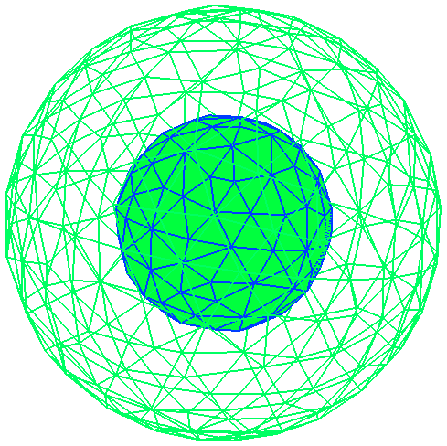
To represent a spherical shell in scuff-em, we need two surface meshes, one each for the inner and outer spherical surfaces. These are described by gmsh mesh files Sphere_R1P0.msh and Sphere_R0P5.msh We describe the shell as an inner vacuum sphere embedded in the outer sphere; the geometry file for this situation is SphericalShell.scuffgeo:

 OBJECT OuterSphere 
     MESHFILE Sphere_R1P0.msh
     MATERIAL CONST_EPS_10
 ENDOBJECT 

 OBJECT InnerSphere 
     MESHFILE Sphere_R0P5.msh
     MATERIAL Vacuum
 ENDOBJECT 

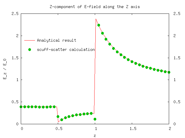
We will run two separate calculations. First, we will fix the relative permittivity of the shell at ε^r=10 and look at the z component of the electric field at points on the z axis ranging from the origin (the center of the concentric spheres) to the exterior medium. We create a file called LineOfPoints which lists the Cartesian coordinates of each evaluation point:

      0.0 0.0 0.000
      0.0 0.0 0.025
      0.0 0.0 0.050
      ...
      0.0 0.0 2.000

We will pass this file to scuff-scatter using the --EPFile option:

     % scuff-scatter --EPFile LineOfPoints < Args

where the Args file looks like this:

      geometry       SphericalShell.scuffgeo
      cache          SphericalShell.cache
      omega          0.001
      pwDirection    1.0 0.0 0.0
      pwPolarization 0.0 0.0 1.0

Note that we choose a frequency low enough to ensure we are well within the electrostatic limit, and that the constant z-directed electrostatic field described in the memo above becomes a linearly polarized plane wave traveling in the x- direction.

This run of the code produces files SphericalShell.scattered and SphericalShell.total. Plotting the 8th vs. the 3rd column of the latter file (look at the first few lines of the file for a description of which column is which) yields plot of the real part of E_z vs. z and yields good agreement with the analytical calculation, modulo some funkiness at points on or near the boundary surfaces which is to be expected in an SIE/BEM calculation:

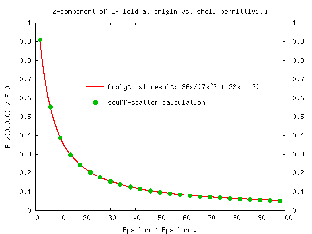
Next, we will vary the shell permittivity and look at the electric field at the center of the shell. In this case the analytical solution makes the interesting prediction

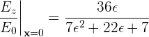
which we will try to verify numerically.

This calculation is slightly trickier than the last one, because scuff-scatter doesn't offer command-line options for varying the dielectric constant of an object. One way around this is to use the python interface to scuff-em, as discussed on this page. Here we will pursue a different solution involving a shell script that modifies the .scuffgeo file for each different value of ε we want to simulate. That script looks like this:

#!/bin/bash

cat EpsValues | while read EPS
do

  # copy the .scuffgeo file with EPS_10 replaced by EPS_xx
  sed "s/EPS_10/EPS_${EPS}/" SphericalShell.scuffgeo > temp.scuffgeo

  # run scuff-scatter to get E-field at origin
  /bin/rm -f CenterPoint.total
  /bin/rm -f CenterPoint.scattered
  scuff-scatter --geometry temp.scuffgeo --EPFile CenterPoint < Args

  # extract the z-component of the field from the output file
  EZ=`awk '{print $8}' CenterPoint.total`
  echo "${EPS} ${EZ}" >> EzVsEps.dat

done

(Here EpsValues is a file containing the values of ε that we want to simulate, and CenterPoint is a file containing just the first line of the file LineOfPoints for the cartesian coordinates of the origin.)

The result of the calculation looks like this:

Comments