Spatially-resolved study of plane-wave transmission through an (infinite-area) thin dielectric film
The previous examples dealt with compact scatterers. We'll next consider an
extended geometry -- namely, a thin dielectric film of
finite thickness in the z direction but infinite extent in the x and y
directions. This is the same geometry for which we used scuff-transmission
to look at the plane-wave transmission and reflection coefficients as a function
of frequency in this example,
but here we'll do a different calculation -- namely, we'll pick a single
frequency and look at how the electric and magnetic fields vary in space,
both inside and outside the thin film. (The files for this example may be
found in the share/scuff-em/examples/ThinFilm directory of your scuff-em
installation.)
The mesh file and .scuffgeo file for this geometry are discussed in the
documentation for scuff-transmission.
The geometry consists of a film of thickness T=1μm, with relative dielectric
constant , illuminated from below by a plane wave at normal
incidence. (We'll take the incident field to be linearly polarized with E field
pointing in the x direction.) The lower and upper surfaces of the film are at
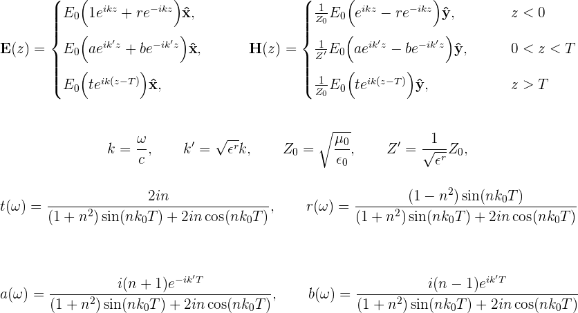
z=0 and z=T. For this geometry it is easy to solve Maxwell's equation directly
to obtain the E and H fields directly at points below, within, and above
the film:
We will try to reproduce this behavior using scuff-scatter.
First create a little text file
(ThinFilm.EvalPoints) containing the
coordinates of a bunch of points on a straight line passing
from below the film to above the film. Then put the following
command-line arguments into a file called ThinFilm_58.args:
 geometry ThinFilm_58.scuffgeo
 cache ThinFilm_58.scuffcache
 omega 1.0
 EPFile ThinFilm.EvalPoints
 pwDirection 0 0 1
 pwPolarization 1 0 0
and pipe it into scuff-scatter:
scuff-scatter < scuff-scatter.args
This produces files named ThinFilm.scattered and
ThinFilm.total. Looking at the first few lines of these
files, we see that the 3rd data column on each line is
the coordinate of the evaluation point, the 4th column
is the real part of , and the 12th column is
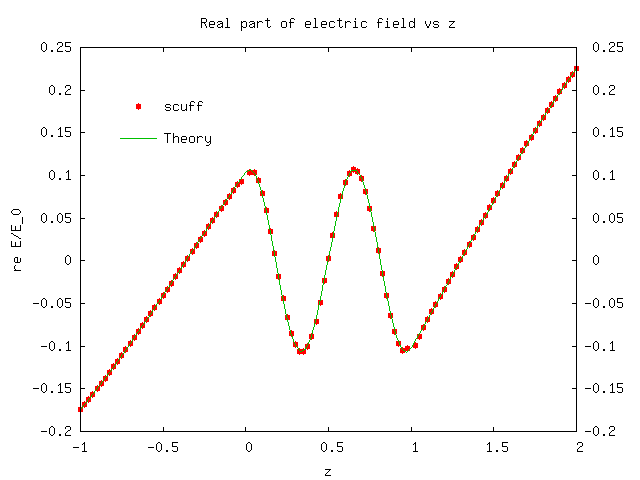
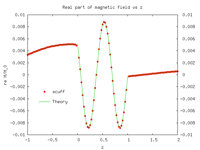
the real part of . Thus, plotting the 4th vs. 3rd
and 12th vs. 3rd columns of the .total file yields plots of
the total
electric and magnetic field vs. , whereupon we find good
agreement with theory: