

S-parameters, directivity, and radiated field patterns of Yagi-Uda antennas

In this example we'll use the scuff-rf application module within the scuff-em suite to investigate a Yagi-Uda antenna design. We will consider both free-standing antennas and antennas printed on PCBs, with the effect of the PCB handled implicitly using scuff-em's support for implicit treatment of multilayer dielectric substrates. We will look at both (a) input impedance vs. frequency, (b) radiation patterns and directivity for antennas driven at a given frequency with given port currents.

The files for this example may be found in the share/scuff-em/examples/YagiUdaAntennas directory of your scuff-em installation.

gmsh geometry and mesh files

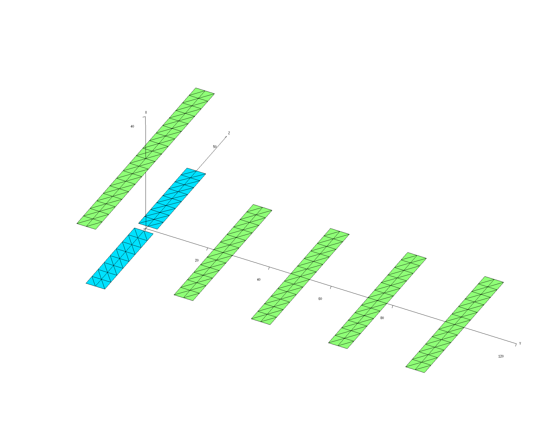
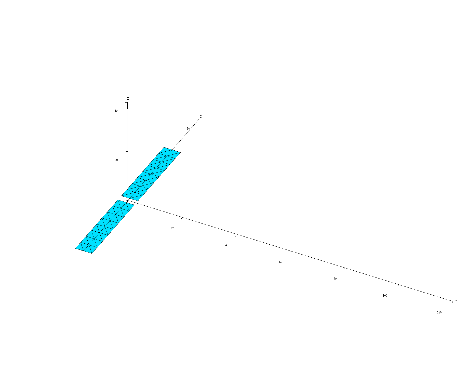
The gmsh geometry file PlanarYUAntenna.geo describes three separate structures: a dipole antenna with a small feed inlet that will be the driven element in our Yagi-Uda antenna, a reflector, and a director.

% gmsh -clscale 1   -2 PlanarYUAntenna.geo -o PlanarYUAntenna_Medium.msh
% gmsh -clscale 0.5 -2 PlanarYUAntenna.geo -o PlanarYUAntenna_Fine.msh

The various scuff-em geometry files below then describe Yagi-Uda antennas consisting of the driven dipole element, optionally with a reflector, and optionally with one or more directors.

• scuff-em geometry file for Yagi-Uda antenna with reflector and 2 directors: YUAntenna_N2_Medium.scuffgeo

• scuff-em geometry file for Yagi-Uda antenna with reflector and 4 directors: YUAntenna_N4_Medium.scuffgeo

• scuff-em geometry file for just the dipole element of the YU antenna alone: DipoleAntenna_Medium.scuffgeo

Visualize scuff-em geometries:

Antenna with $N=2$ directors:

% export SCUFF_MESH_PATH=./mshFiles
% scuff-analyze --geometry scuffgeoFiles/YUAntenna_N2_Medium.scuffgeo --WriteGMSHFiles
% gmsh YUAntenna_N2_Medium.pp

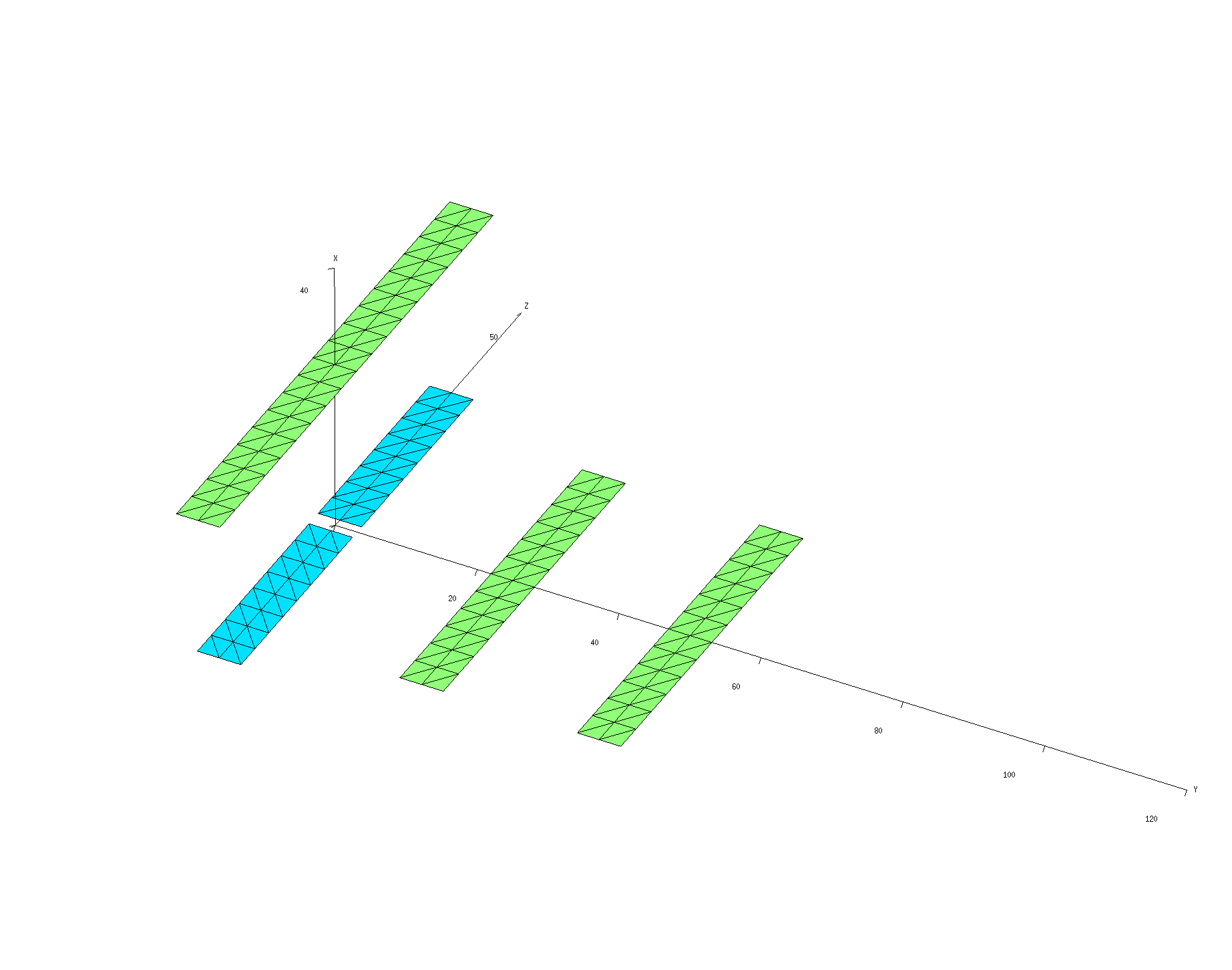
Antenna with $N=4$ directors:

% export SCUFF_MESH_PATH=./mshFiles
% scuff-analyze --geometry scuffgeoFiles/YUAntenna_N4_Medium.scuffgeo --WriteGMSHFiles
% gmsh YUAntenna_N4_Medium.pp

Just the dipole element in isolation:

% export SCUFF_MESH_PATH=./mshFiles
% scuff-analyze --geometry scuffgeoFiles/DipoleAntenna_Medium.scuffgeo --WriteGMSHFiles
% gmsh DipoleAntenna_Medium.pp

Port file

The file Dipole.ports specifies the RF ports of the structure; in this case there is just one port, whose positive and negative terminals are the upper and lower edges of the feed gap in the driven dipole element.

To verify that scuff-rf interprets the .ports file correctly to describe the actual ports we intended, we do a quick run of scuff-rf with the --PlotPorts option:

 % export SCUFF_MESH_PATH=./mshFiles
 % scuff-rf --geometry scuffgeoFiles/YUAntenna_N2_Medium.scuffgeo --PortFile portFiles/Dipole.ports --PlotPorts
 % gmsh YUAntenna_N2_Medium.pp YUAntenna_N2_Medium.ports.pp

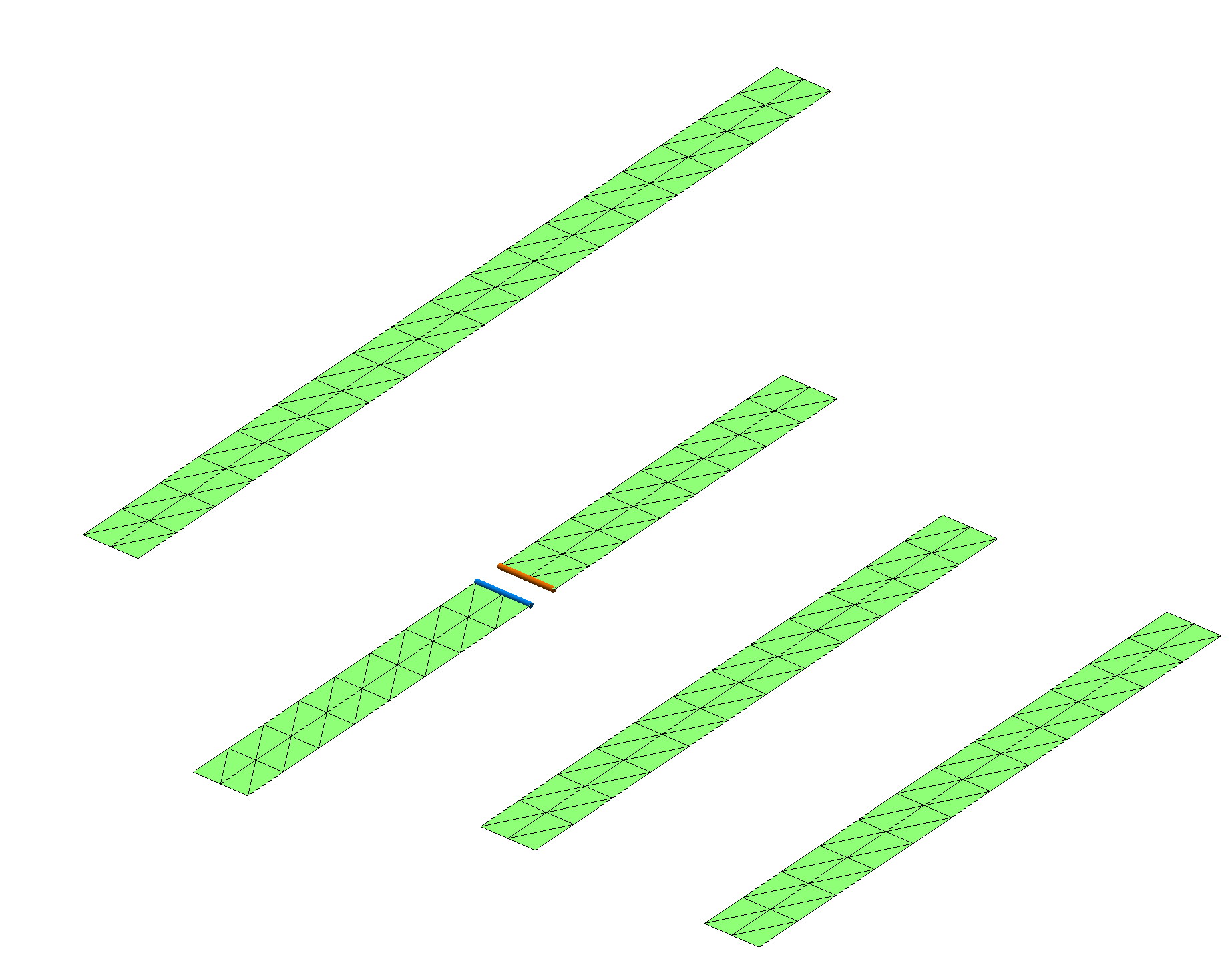
The red- and blue-highlighted regions of the structure are the positive and negative terminals of the port.

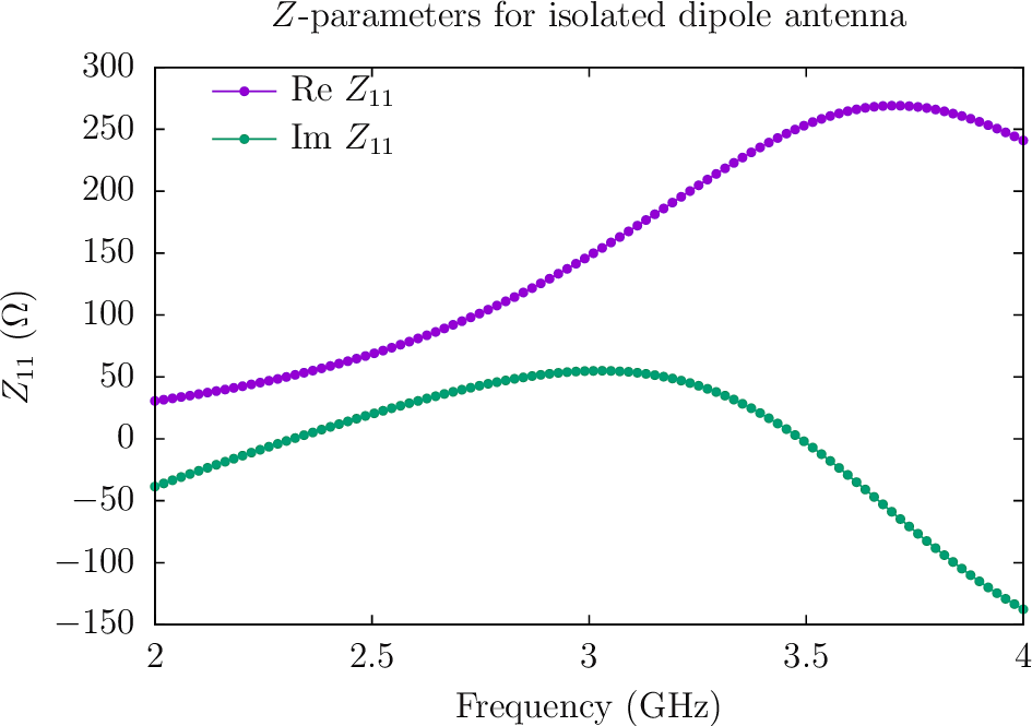
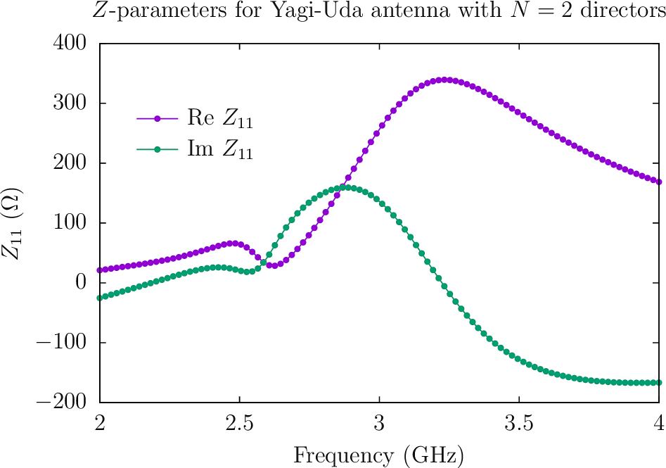
First run to compute $S$- and $Z$-parameters

The simple shell script RunScript.SZParms computes $S$- and $Z$-parameters for the various structures over a range of frequencies. I plot the results in gnuplot using this script: Plotter.zparms.

 % RunScript.SZParms
 % gnuplot
 gnuplot> load 'Plotter.zparms'

Second run to compute radiation patterns

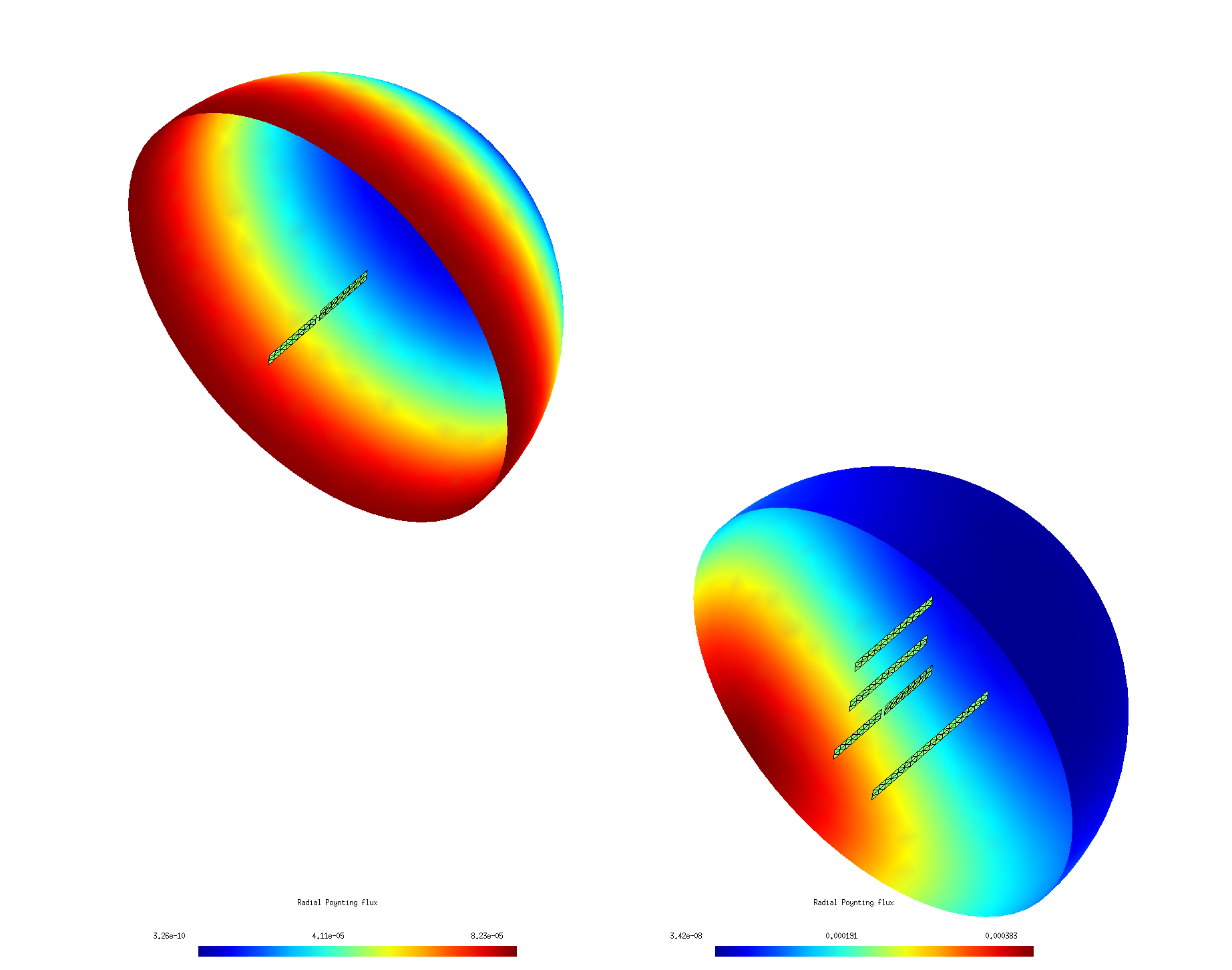
Based on the $Z$-parameter data, it looks like the $N=2$ Yagi antenna wants to radiate at a frequency around 3.2 GHz. So let's drive the antenna with a unit-strength current at that frequency and visualize the resulting radiation patterns by plotting outgoing Poynting flux on a hemispherical surface. The simple shell script RunScript.FieldPatterns does this for the various antennas:

#!/bin/bash

CODE=scuff-rf

BASE=.
export GEODIR=${BASE}/scuffgeoFiles
export SCUFF_MESH_PATH=${BASE}/mshFiles

ARGS=""
ARGS="${ARGS} --portfile ${BASE}/portFiles/Dipole.ports"
ARGS="${ARGS} --portcurrentFile ${BASE}/portcurrentFiles/Dipole.PortCurrents"
ARGS="${ARGS} --FVMesh Hemisphere.msh"

for GEOM in DipoleAntenna YUAntenna_N2 YUAntenna_N4
do
  ${CODE} ${ARGS} --geometry ${GEODIR}/${GEOM}_Medium.scuffgeo
done

Notes:

• The file Dipole.PortCurrents is a list of frequencies at which to run calculations and the currents to force into each port at those frequencies. For a geometry with $N$ ports, each line of this file has $2N+1$ columns: the frequency in GHz followed by the real and imaginary parts of the current to force into each port. For the case at hand, we want to run at just the single frequency $f$=3.2 GHz with a unit-strength current forced into port 1, so the .PortCurrents file looks simply like

 3.2 1.0 0.0

• The field-visualization mesh Hemisphere.msh is a gmsh surface mesh produced from the gmsh geometry file Hemisphere.geo. You can get higher-resolution images by meshing this file with higher resolution.

Running the above script produces files with names like YUAntenna_N2_Medium.Hemisphere.pp showing outgoing Poynting flux plotted over the hemisphere mesh. Here's a composite image showing results for the isolated dipole and the $N=2$ Yagi-Uda antennas, with the antenna meshes superposed (and enlarged by a factor of 5× to make it easier to see them). The simple dipole antenna radiates isotropically, while the Yagi antenna exhibits high directivity.

Python-driven directivity optimization

Comments