

Dyadic Green's Functions and LDOS above a material half-space

In this example, we exploit scuff-em's support for 2D periodic geometries by using scuff-ldos to compute dyadic Green's functions (DGFs) and electromagnetic local densities of states (LDOS) at evaluation points lying above an infinite planar dielectric interface.

Because this geometry happens to be amenable to an analytical treatment, we will also check the numerical results of scuff-em against the results of analytical calculations of the LDOS.

The files for this example may be found in the share/scuff-em/examples/HalfSpaceLDOS subdirectory of your scuff-em installation.

Review: What we are computing and why we need Brillouin-zone integration

For the benefit of users who may be wondering why numerical Brillouin-zone integration is needed for this calculation, this section briefly reviews some of the theoretical background. (This material is discussed in more detail in the memo Computation of Green's Functions and LDOS in scuff-em). If you just want to get started running the calculations in scuff-em, feel free to skip to the next section.

Green's functions and LDOS

The scattering dyadic Green's function $\boldsymbol{\mathcal G}^{\text E}(\omega; \mathbf{x}_{\text D}, \mathbf{x}_{\text S})$ of a material geometry is a $3\times 3$ matrix whose $i,j$ entry is proportional to the $i$ -component of the scattered electric field at $\mathbf{x}_{\text D}$ due to a $j$ -directed point electric dipole source at $\mathbf{x}_{\text S}$ , all quantities having time dependence $\sim e^{-i\omega t}$ . (We could also consider the magnetic Green's function $\boldsymbol{\mathcal G}^{\text M}$ , which describes the scattered magnetic fields arising from a point magnetic dipole excitation.) The subscripts "D" and "S" label the "destination" and "source" points; if these coincide $(\mathbf{x}_{\text D}=\mathbf{x}_{\text S})$ , we are talking about one-point DGFs; otherwise we have two-point DGFs.

The one-point scattering DGFs for a material geometry contain information on how the bodies in the geometry modify the electromagnetic local density of states (LDOS) in the vicinity of the body. More specifically, the full LDOS $\rho(\mathbf{x})$ at a point $\mathbf{x}$ may be decomposed as a sum of electric and magnetic contributions, which themselves may be further decomposed into vacuum and scattering contributions: $\begin{array}{lcl} \rho(\omega; \mathbf{x}) &=& \rho^\text{E}(\omega; \mathbf{x}) + \rho^\text{M}(\omega; \mathbf{x}) \\[5pt] \rho^{\text{E,M}}(\mathbf{x}) &=& \rho_0(\omega) + \Delta \rho^\text{E,M}(\omega; \mathbf{x}) \\[5pt] \rho_0(\omega) &=&\frac{\omega^2}{\pi^2 c^3} \\[5pt] \Delta \rho^{\text{E,M}}(\omega; \mathbf{x}) &=& \frac{\omega}{\pi c^2} \text{Tr Im }\boldsymbol{\mathcal{G}}^\text{E,M}(\omega; \mathbf{x}, \mathbf{x}) \end{array}$

Computing Green's functions

The electric and magnetic DGFs for a given source point (and any number of destination points) collectively describe the results of 6 scattering problems (with incident fields produced by electric and magnetic dipoles oriented in each of the 3 cartesian directions), and---for compact geometries---could be computed in scuff-em simply by assembling 6 right-hand-side vectors, solving the BEM system for the corresponding surface currents, and computing the scattered fields at all desired destination points.

However, the situation is more complicated for infinitely extended geometries. Recall that such geometries are described in scuff-em by a unit-cell geometry together with a basis of vectors for a (one- or two-dimensional) lattice $\mathcal{L}$ . By restricting our attention to scattering problems in which the incident fields (and thus all fields and currents) satisfies the Bloch-periodicity condition $f(\mathbf{x}+\mathbf{L}) = e^{i\mathbf{k}_\text{B}\cdot \mathbf{L}}f(\mathbf{x}) \quad\text{ for all } \quad \mathbf{L}\in\mathcal{L}$ for some Bloch wavevector $\mathbf{k}_\text{B}$ , we can get away with solving only for the surface currents within the unit cell, the currents everywhere else being then fixed by the Bloch periodicity. This is the basic magic trick that allows infinite geometries to be modeled on finite computers.

Of course, the restriction to scattering problems involving only Bloch-periodic incident fields is in fact highly restrictive; indeed, it excludes the particular problem we must solve to compute DGFs and LDOS, in which the incident field emanates from a point source at $\mathbf{x}_\text{S}$ and is certainly not Bloch-periodic. But here we can avail to the linearity of Maxwell's equations and the magic of Fourier analysis. Instead of solving a scattering problem involving the field of a point source at $\mathbf{x}_\text{S}$ , we consider the field of an infinite phased array of point sources, located at points $\{\mathbf{x}_\text{S} + \mathbf{L}\}$ with phases $e^{i\mathbf{k}_\text{B} \cdot \mathbf{L}}$ , for all $\mathbf{L}\in \mathcal{L}$ . This is a Bloch-periodic field, so we can take it as the incident field in a scuff-em scattering problem, and the resulting scattered fields at $\mathbf{x}_\text{D}$ define the Bloch-periodic scattering DGFs $\overline{\boldsymbol{\mathcal{G}}}(\omega; \mathbf{k}_\text{B}; \mathbf{x}_\text{D}, \mathbf{x}_\text{S}).$ To recover the non-periodic DGF $\boldsymbol{\mathcal{G}}$ from $\overline{\boldsymbol{\mathcal{G}}}$ , we now imagine solving and summing the results of many scattering problems involving our infinite array of point sources phased with many different Bloch vectors $\mathbf{k}_\text{B}$ , chosen cleverly to ensure that the contributions of the single point source at $\mathbf{x}_\text{S}$ add constructively, while the contributions of all other point sources in the array add destructively and cancel. The formal expression of this procedure is a sort of inverse Fourier transform relating $\boldsymbol{\mathcal{G}}$ to the average of $\overline{\boldsymbol{\mathcal{G}}}(\mathbf{k}_\text{B})$ over the Brillouin zone (BZ) of the reciprocal lattice: $\boldsymbol{\mathcal G}(\omega; \mathbf{x}_\text{D}, \mathbf{x}_\text{S}) =\frac{1}{V_\text{BZ}} \int_\text{BZ} \overline{\boldsymbol{\mathcal G}}(\omega; \mathbf{k}_\text{B}; \mathbf{x}_\text{D}, \mathbf{x}_\text{S}) \, d\mathbf{k}_\text{B} \qquad (1)$ or, evaluating the integral approximately by numerical cubature, $\boldsymbol{\mathcal G}(\omega; \mathbf{x}_\text{D}, \mathbf{x}_\text{S}) \approx \frac{1}{V_\text{BZ}} \sum_{m} w_m \overline{\boldsymbol{\mathcal G}}(\omega; \mathbf{k}_{\text{B}m}; \mathbf{x}_\text{D}, \mathbf{x}_\text{S})$ where $\{\mathbf{k}_{\text{B}m}, w_m\}$ are the points and weights in a cubature rule for integration over the Brillouin zone. Thus, getting the LDOS at a single point in a periodic geometry requires summing the results of many scattering calculations at various Bloch vectors $\mathbf{k}_{\text{B}m}$ lying in the Brillouin zone of the reciprocal lattice.

The question of how to choose the cubature rule---that is, the set of Bloch vectors $\{\mathbf{k}_{\text{B}m}\}$ at which the integrand is sampled and the weights $\{w_m\}$ with which the samples are combined---to yield accurate integral estimates without exorbitant computational cost is a tricky one, and one whose answer varies from problem to problem. There are two ways to proceed:

You can design your own cubature scheme for integration over the Brillouin zone, and simply ask scuff-ldos to give you values of the integrand $\overline{\boldsymbol{\mathcal{G}}}(\mathbf{k}_\text{B})$ at specific Bloch vectors $\bf k_\text{B}$ . In this case you will pass the --OmegakBlochFile command-line argument to scuff-ldos, and you will get back a data file (with extension .byOmegakBloch) reporting values of $\overline{\boldsymbol{\mathcal{G}}}$ at each $\bf k_\text{B}$ point you specified. (See below for examples).

Alternatively, you can use the built-in Brillouin-zone integrator in scuff-ldos to perform the BZ integral automatically. In this case you will get back a data file with extension .LDOS reporting values of $\boldsymbol{\mathcal{G}}$ and $\Delta\rho$ at each frequency and evaluation point you specified, plus a data file with extension .byOmegakBloch reporting the Bloch vectors $\bf k_\text{B}$ at which the internal integrator sampled the integrand and the values of $\overline{\boldsymbol{\mathcal{G}}}(\bf k_\text{B})$ at each sample point. In this case you will probably want to set various command-line options to optimize the integral evaluation; this is illustrated below and discussed in more detail on the page Brillouin-zone integration in scuff-em.

gmsh geometry files for unit-cell geometries

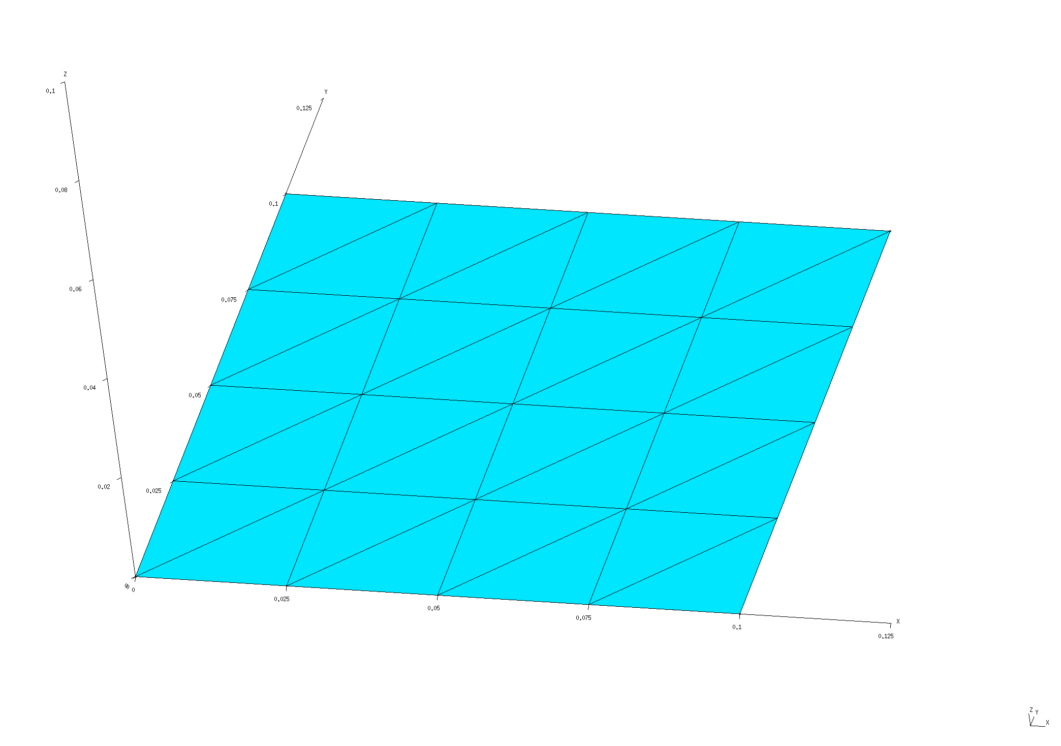
To compute DGFs and LDOS in a half-space geometry, we will describe the interface between the upper (vacuum) and lower (dielectric) regions of our geometry as the infinite periodic replication of a unit-cell mesh over the sites of a 2D square lattice. Because this particular geometry has infinite translational symmetry, we are free to choose the lattice constant $L=L_x=L_y$ however we like; here we will consider the two values $L=10$ nm and $L=100$ nm.

The gmsh geometry file Square_L_N.geo describes a square with user-adjustable parameters L and N that may be configured using the -setnumber option on the gmsh command line to define the square side length and the number of triangle edges per side length (the meshing fineness). To produce unit-cell meshes for the two desired lattice constants, I go like this:

% gmsh -2 -setnumber L 0.1 -setnumber N 4 Square_L_N.geo -o Square_L0P1.msh 
% RenameMesh Square_L0P1.msh

% gmsh -2 -setnumber L 0.01 -setnumber N 4 Square_L_N.geo -o Square_L0P01.msh 
% RenameMesh Square_L0P01.msh

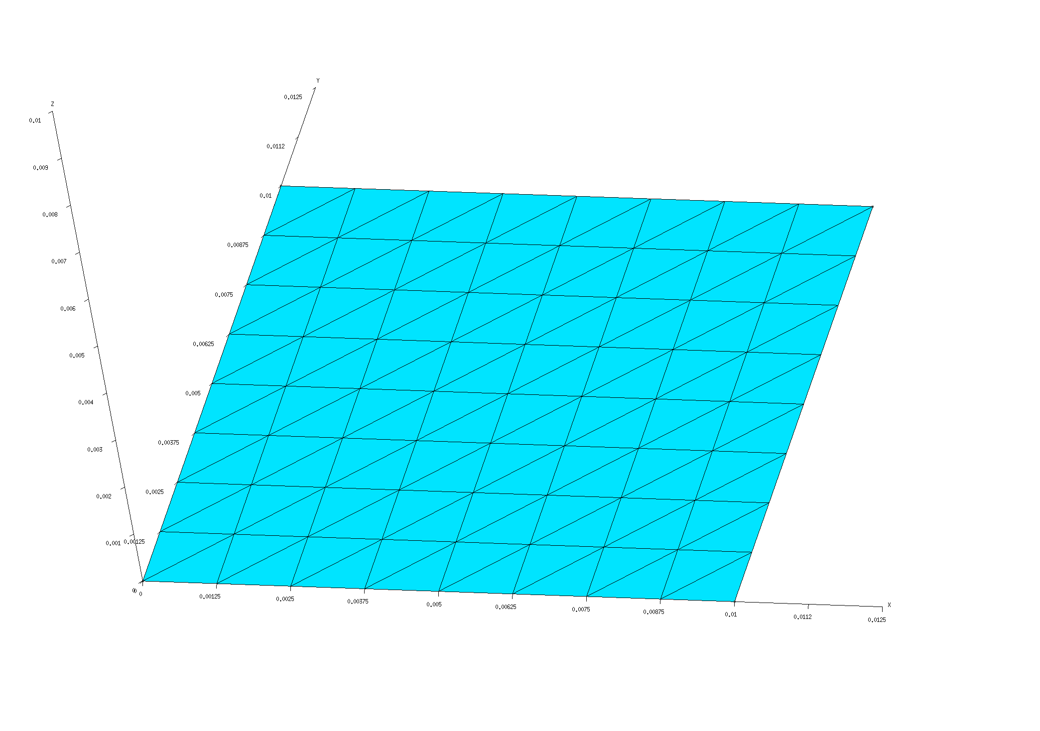
(Here RenameMesh is a simple bash script that uses scuff-analyze to count the number of interior edges in a surface mesh and rename the mesh file accordingly.) These commands produce the files Square_L0P1_40.msh and Square_L0P01_40.msh. I also repeat the process with -setnumber N 8 to yield finer meshes (with 176 instead of 40 interior edges). These meshes may be visualized in gmsh by saying e.g.

% gmsh Square_L0P1.40.msh
% gmsh Square_L0P01.176.msh

Note the following:

For 2D periodic geometries in scuff-em, the lattice vectors must lie in the $xy$ plane.
For surfaces that straddle the unit-cell boundaries (as is the case here), each triangle edge that lies on any edge of the unit cell must have an identical image edge on the opposite side of the unit cell. An easy way to achieve this is to use extrusions in gmsh, as in the .geo file above.
Among the various possible ways to discretize a square intro triangles, I have chosen one that preserves as much symmetry as possible---specifically, the mesh is symmetric under the transformations $x \leftrightarrow -x$ , $y \leftrightarrow -y$ , and $x \leftrightarrow y$ . This is important for exploiting symmetries to reduce the cost of Brillouin-zone integration (see below).

The .msh files needed to run the calculations in this tutorial may be found in the mshFiles/ subfolder of the HalfSpaceLDOS example distributed with scuff-em.

scuff-em geometry files

For each unit-cell mesh I create scuff-em geometry files describing three material geometries:

an infinite-area perfectly electrically conducting (PEC) plate at height $z=0$ ;
an infinite lossless dielectric ( $\epsilon \equiv 10$ ) filling space for $z<0$ , with vacuum for $z>0$ ;
same as previous, but now with lossy metal (aluminum) instead of lossless dielectric.

The resulting .scuffgeo files may be found in the scuffgeoFiles/ subfolder of the HalfSpaceLDOS example directory. For example, the PEC-plate geometry at the coarser resolution with the longer lattice constant is PECPlate_L0P1_40.scuffgeo, while the aluminum half-space geometry at the finer resolution with the shorter lattice constant is AlHalfSpace_L0P01_176.scuffgeo. The latter file looks like this:

# this comes from Phys Rev B **68** 245405
MATERIAL ALUMINUM
    wp = 1.747e16; 
    gamma = 7.596e13;
    Eps(w) = 1 - wp^2 / (w * (w + i*gamma));
ENDMATERIAL

LATTICE
    VECTOR 0.01 0.00
    VECTOR 0.00 0.01
ENDLATTICE

REGION UpperHalfSpace MATERIAL Vacuum
REGION Exterior       MATERIAL Aluminum

SURFACE Plate
    MESHFILE Square_L0P01_176.msh
    REGIONS Exterior UpperHalfSpace
ENDSURFACE

List of evaluation points

We'll compute one-point DGFs and LDOS at four points, located at distances of 1, 10, 100, and 1000 nm above the surface on the $z$ -axis ( $x=y=0$ ). Thus our evaluation-point file (EPFile) looks like this:

0.0 0.0 0.001
0.0 0.0 0.010
0.0 0.0 0.100
0.0 0.0 1.000

Studying the integrand to select the optimal cubature rule

Ultimately we will want to launch a full Brillouin-zone-integrated calculation to get the total LDOS at our desired evaluation points and frequencies. However, before doing this we should acquire some insight into the behavior of the integrand so that we can make intelligent choices for the various options controlling Brillouin-zone integration.

Checking Brillouin-zone symmetry

A first thing to check is the symmetry of the integrand within the Brillouin zone (BZ). As discussed here, the built-in cubature routines for 2D BZ integration in scuff-em can exploit 2, 4, or 8-fold rotational symmetry. In this case, because

(1) the underlying (real-space) geometry is symmetric under $x\leftrightarrow -x$ , $y\leftrightarrow -y$ , and $x\leftrightarrow y$ ,
(2) we have chosen a mesh discretization that preserves these symmetries, and
(3) we are computing a one-point DGF,

we expect the BZ integrand $\overline{\boldsymbol{\mathcal{G}}}(k_x,k_y)$ to have 8-fold rotational symmetry, and thus we should be able to restrict the domain of the BZ integration to just the irreducible Brillouin zone (a triangular wedge having 1/8 the total area of the BZ, as shown here) and multiply by 8 to get the full BZ integral.

To test this, we'll run a quick first calculation in which we compute just the integrand $\boldsymbol{\mathcal{G}}(k_x,k_y)$ at 8 $(k_x,k_y)$ points related by symmetry. Specifically, for a square lattice with lattice constant $L=100\text{ nm}$ (reciprocal lattice constant $\Gamma=\frac{2\pi}{100\text{ nm}}$ ) we'll consider the point $(k_x,k_y)=(0.40\Gamma,0.27\Gamma)\approx(25,17)\,\mu\text{m}^{-1}$ and the 7 other points obtained by flipping signs and interchanging components. Here's a picture showing the locations of these 8 points within in the BZ:

Working at angular frequency $\omega=10 \cdot 3\times 10^{14}$ rad/sec, we create a little text file named EightPoints listing the $(\omega, k_x, k_y)$ values at which we want to sample the BZ integrand:

Now run scuff-ldos:

% scuff-ldos --geometry scuffgeoFiles/AlHalfSpace_L0P1_40.scuffgeo --OmegakBlochFile EightPoints --EPFile EPFile

This produces the file AlHalfSpace_L0P1_40.byOmegakBloch, in which each individual line reports $\overline{\mathcal{G}}$ values for a single evaluation point, frequency, and Bloch vector. Looking at just the portion of the file corresponding to the evaluation point at $z=100$ nm, we see this:

This shows that, as expected, the Brillouin-zone integrands for the electric and magnetic LDOS $\rho^\text{E,M}$ are invariant---up to small numerical errors on the order of around 1%, which are reduced to around 0.1% when we re-run the calculation on the finer [N=176] mesh---under the 8-fold symmetry relating the various Brillouin-zone points here. Later we will exploit this symmetry by specifying the command-line option --BZSymmetryFactor 8 to reduce the cost of evaluating the full BZ integral.

Incidentally, notice that the individual components of the DGFs (such as $\overline{\mathcal{G}}_{xx}$ ) do not obey the full set of symmetries obeyed by the LDOS. You will need to take this into account if your goal is to compute DGFs and not just LDOS.

Observing the variation of the integrand with $|\mathbf{k}_\text{B}|$

Another diagnostic test is to inspect the variation of the integrand with the magnitude of the Bloch vector. For this purpose we'll compute the integrand at points lying on the $x$ -axis between the origin and the edge of the BZ, again working with the $L=100$ nm lattice at $\omega=10$ . We create a file called XAxisPoints specifying the ( $\omega,k_x,k_y$ ) points we want to sample:

10  00.0  0.0
10  1.57  0.0
10  3.14  0.0
...
10  29.8  0.0
10  31.4  0.0

Run scuff-ldos:

% scuff-ldos --geometry scuffgeoFiles/AlHalfSpace_L0P1_40.scuffgeo --OmegakBlochFile XAxisPoints --EPFile EPFile

This produces the file AlHalfSpace_L0P1_40.byOmegakBloch. We plot the BZ integrand for the electric LDOS $\rho^\text{E}(\mathbf{k})$ versus $k_x$ at $z=100$ nm:

% gnuplot
gnuplot> FILE='AlHalfSpace_L0P1_40.byOmegakBloch'
gnuplot> set yrange [-100:100]
gnuplot> plot FILE u ($3==0.1 ? $6 : 1/0):8 w lp pt 7 ps 1

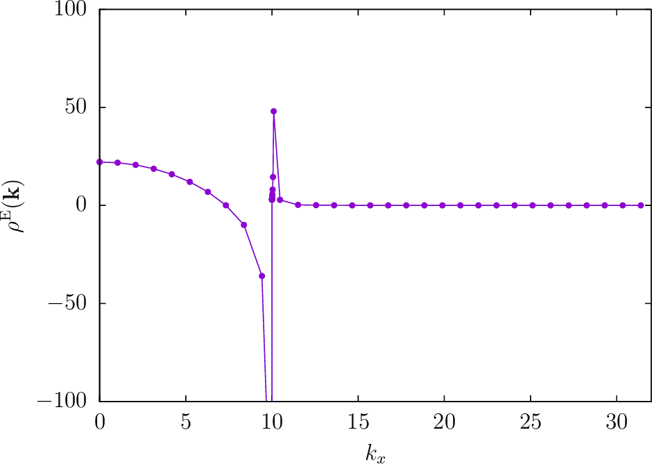
Whoops! There seems to be some sort of blowup happening near $k_x=10$ , i.e. near the point $k_x=\frac{\omega}{c}$ where the Bloch wavelength coincides with the free-space photon wavelength. Zooming in on the region near $k_x=10$ , the data look like this (where we have additionally plotted data for evaluation points at a couple of other heights off the surface):

The important things to read off from this plot are:

As $|\mathbf{k}_\text{B}|\to k_0\equiv \frac{\omega}{c}$ from below, the integrand blows up like $1/\sqrt{k_0 - |\mathbf{k}_\text{B}|}.$
On the other side of $k_0$ , the integrand decays exponentially at a $z$ -dependent rate.

This behavior is expected for cases in which the photon wavenumber lies within the Brillouin zone; the square-root blowup in the LDOS is just the usual van Hove singularity, while the exponential decay for larger $k$ arises because plane waves with transverse wavelength shorter than the free-space photon wavelength are evanescent (not propagating) waves that decay exponentially with distance from the surface.

(BTW, here is the gnuplot script that produces the two plots above.)

Running full Brillouin-zone-integrated calculations

Now it's time to launch runs for full BZ-integrated LDOS. For this purpose we will want to set appropriate values for the command-line options controlling Brillouin-zone integration. We have already determined that the integrand has 8-fold symmetry, so we will be specifying --BZSymmetryFactor 8. The next task is to choose a cubature rule ("BZ integration method"), i.e. a strategy for sampling the integrand at appropriately-chosen $|\mathbf{k}_\text{B}|$ points to estimate the integral accurately with as few samples as possible.

The presence of the $|\mathbf{k}_\text{B}|=k_0$ singularity in the Brillouin zone makes this a good candidate for the Polar2 strategy, which performs the BZ integral using a polar decomposition $\mathbf{k}_\text{B}=(k_\rho, k_\theta)$ , with the integrals over the regions $k_\rho < k_0$ and $k_\rho>k_0$ handled separately, and with the change of variables $k_\rho \to k_z=\sqrt{|k_0^2 - k_\rho^2|}$ to neutralize the square-root singularity at $k_\rho = k_0.$ In this case the integrals over $k_z$ and $k_\theta$ are performed using $N_\rho$ and $N_\theta$ evaluation points, respectively, where $N_\rho$ and $N_\theta$ are combined into a single value specified as the --BZIOrder command-line option, i.e. $\texttt{--BZIOrder} = N_\rho \times 100 + N_\theta.$ For example, to use 31 points for the radial integral and 11 points for the $\theta$ integral, we would say --BZIOrder 3111.

(Actually, in this particular case, we expect to have full rotational symmetry, i.e. the integrand should be independent of $k_\theta$ , and thus we can specify the special value $N_\theta=2$ to request that the $k_\theta$ integral be evaluated by a one-point cubature sampling just the point $k_\theta=0$ .)

Choosing an 11-point integration rule for the radial integral and the above-discussed 1-point cubature for the $\theta$ integral, our scuff-ldos command-line looks like this:

% scuff-ldos --geometry scuffgeoFiles/AlHalfSpace_L0P1_40.scuffgeo --OmegaFile OmegaFile --EPFile EPFile --BZIMethod Polar2 --BZIOrder 1102

As a comparison, I will also run calculations with $N_\rho=0$ . This selects an adaptive integration algorithm for the radial integral, which determines the number and location of the sample points automatically to achieve user-specified relative and absolute error tolerances, which are set with the --BZIRelTol and --BZIAbsTol command-line options:

% scuff-ldos --geometry scuffgeoFiles/AlHalfSpace_L0P1_40.scuffgeo --OmegaFile OmegaFile --EPFile EPFile --BZIMethod Polar2 --BZIOrder 0002 --BZIRelTol 1.0e-2 --BZIRelTol 1.0e-8

I also run calculations on the finer-resolution mesh (the _176.scuffgeo files) and the mesh with lattice constant $L=0.01\,\mu\text{m}$ (the L0P01 files).

Here's a plot of the LDOS enhancement at $z=10 nm$ :

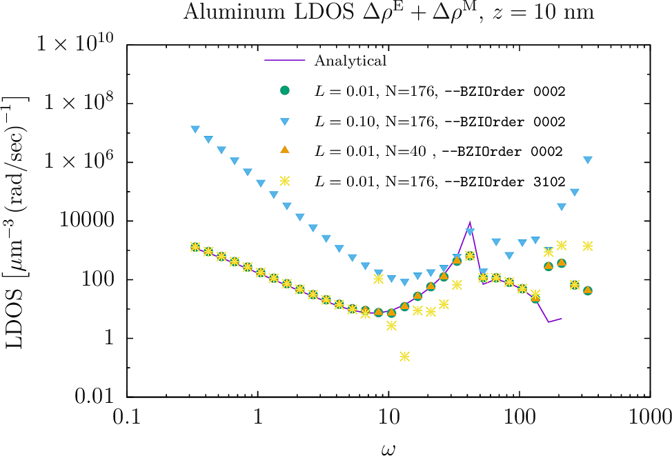
The green dots are for the calculation with all numerical resolution parameters set to their maximum (most accurate and most expensive) values: finest mesh, smallest lattice constant, and adaptive BZ cubature. These points agree well with the analytical prediction up to the highest frequencies, where they start to deviate.

The other data symbols are the results of calculations in which one fineness parameter is relaxed to a less-expensive value:

The blue triangles are for the geometry with lattice constant $L=100$ nm (but still using a fine mesh with adaptive cubature). Evidently this degrades the quality of the numerical data completely. That makes sense, since the evaluation point is at a height $z=10$ nm above the surface. For larger $z$ values the data values for the two lattice constants are in better agreement.

The orange triangles are for the geometry with lattice constant $L=10$ nm, but now meshed at coarser resolution (resulting in $N=40$ triangle edges instead of $N=176$ for the finer case). Evidently this doesn't degrade the quality of the data at all, so for this case we can run calculations with the (significantly cheaper) coarser mesh at no cost in accuracy.

The yellow stars are for the $L=10$ nm geometry with the fine ( $N=176$ ) mesh resolution, but with the BZ integration performed using a fixed-order numerical integration ( $N_\rho=31$ samples) instead of adaptive quadrature for the radial part of the BZ integral. Evidently this yields data that agree with the more accurate adaptive-quadrature data at most frequencies, but deviate over a range of frequencies in the range $\omega\in[10,40]$ and again at high frequencies.