

Electrostatic fields of an electrode array

In this example we use scuff-static to compute the electrostatic fields in the vicinity of a complicated electrode array with the various electrodes held at various external potentials.

More specifically, the calculation will proceed in two stages:

First, for each of the N electrodes in the device we will compute the fields produced by maintaining that electrode at a potential of 1 volt, with all other electrodes grounded. This will produce N separate datasets, each reporting the electrostatic potential and E-field components at our desired evaluation points. The structure of the boundary-element-method (BEM) solver implemented by scuff-static ensures that this calculation is fast, even for large N: once we have assembled and factorized the BEM matrix for a given geometry, we can solve any number of electrostatic problems involving different excitations of that geometry essentially "for free."
Then we will run a second calculation in which all electrodes are maintained at specific voltages and---in addition---an externally-sourced electrostatic field is present. For this case we will generate graphic visualization files illustrating the fields in the vicinity of the device.

The geometry considered in this example is a model of a Paul trap; I am grateful to Anton Grounds for suggesting this application and for providing the sophisticated parameterized gmsh file describing the geometry.

The files for this example may be found in the share/scuff-em/examples/PaulTrap subdirectory of your scuff-em installation.

gmsh geometry and mesh files

The gmsh geometry file Trap.geo describes a collection of conductor surfaces constituting a Paul trap. This file contains a user-specifiable parameter ELCNT that may be used to set the number of electrodes; to create a mesh for a 8-electrode geometry, we say

% gmsh -2 -setnumber ELCNT 4 Trap.geo -o Trap_4.msh

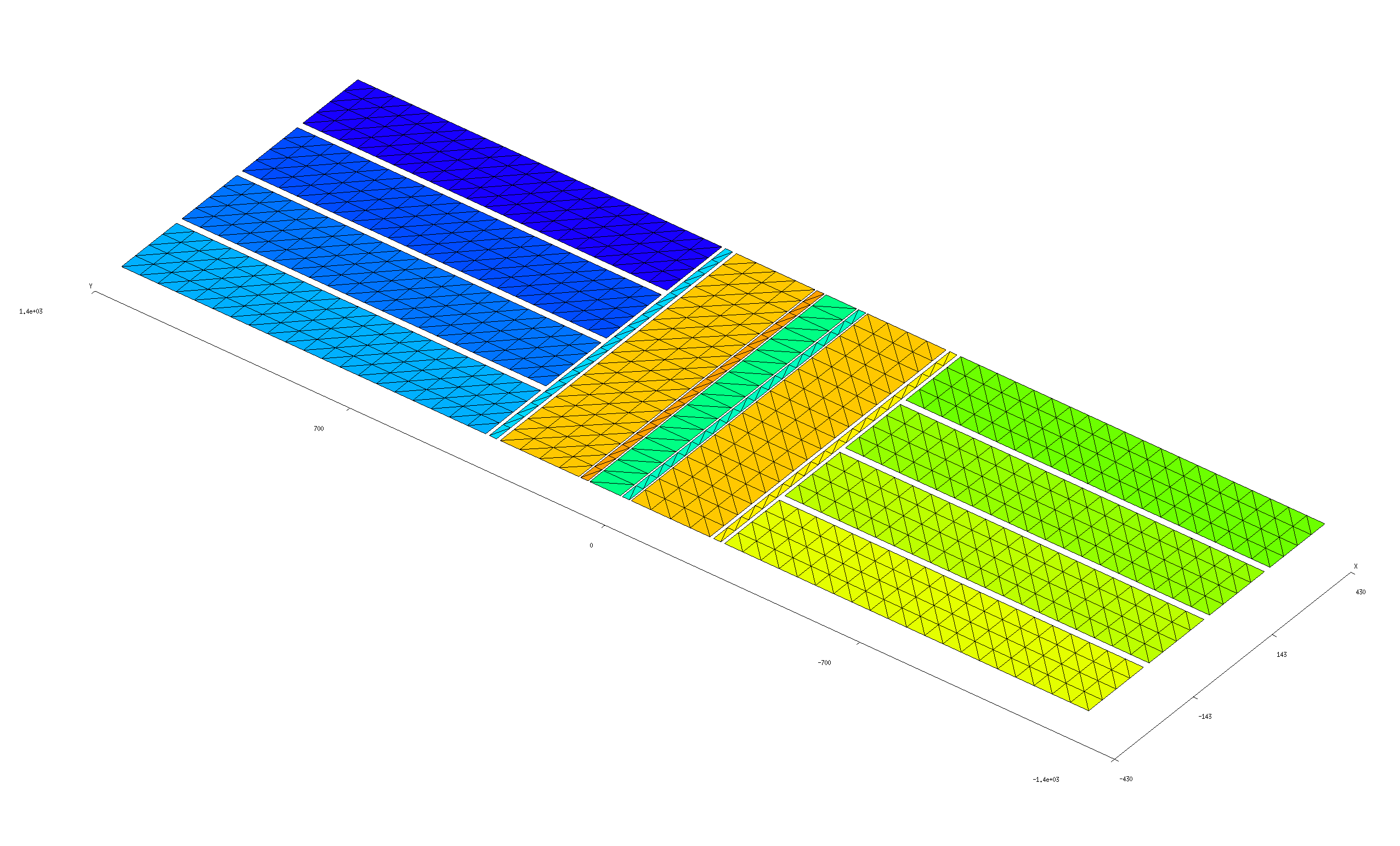
(Note that the total number of electrodes is twice the value specified for ELCNT). This produces the gmsh mesh file Trap_4.msh, which we can open in gmsh to visualize:

% gmsh Trap_4.msh

Trap_4.msh image

Simple scuff-em geometry file

The gmsh file Trap.geo is designed to ensure that each separate metallic strip in the geometry---including each of the 8 identically-shaped electrodes, plus each of the 7 strips of varying thicknesses running down the center of the structure---is meshed as a separate entity and assigned a unique (integer) identifier. Thus, one way to write a scuff-em geometry file for this geometry would be simply to include each of the 15 distinct surfaces in OBJECT...ENDOBJECT clauses, each clause referencing a unique entity in the mesh. This strategy is pursued by the file Trap_4.scuffgeo, which looks like this:

OBJECT GND
    MESHFILE Trap_4.msh
    MESHTAG 1
ENDOBJECT

OBJECT Rot2
    MESHFILE Trap_4.msh
    MESHTAG 2
ENDOBJECT

OBJECT Rot3
    MESHFILE Trap_4.msh
    MESHTAG 3
ENDOBJECT

OBJECT RF
    MESHFILE Trap_4.msh
    MESHTAG 4
ENDOBJECT

OBJECT Rot1
    MESHFILE Trap_4.msh
    MESHTAG 5
ENDOBJECT

OBJECT Rot4
    MESHFILE Trap_4.msh
    MESHTAG 6
ENDOBJECT

OBJECT UpperDC1
    MESHFILE Trap_4.msh
    MESHTAG 7
ENDOBJECT

OBJECT LowerDC1
    MESHFILE Trap_4.msh
    MESHTAG 8
ENDOBJECT

OBJECT UpperDC2
    MESHFILE Trap_4.msh
    MESHTAG 9
ENDOBJECT

OBJECT LowerDC2
    MESHFILE Trap_4.msh
    MESHTAG 10
ENDOBJECT

OBJECT UpperDC3
    MESHFILE Trap_4.msh
    MESHTAG 11
ENDOBJECT

OBJECT LowerDC3
    MESHFILE Trap_4.msh
    MESHTAG 12
ENDOBJECT

OBJECT UpperDC4
    MESHFILE Trap_4.msh
    MESHTAG 13
ENDOBJECT

OBJECT LowerDC4
    MESHFILE Trap_4.msh
    MESHTAG 14
ENDOBJECT

Note that, although each of the OBJECT clauses references the same mesh file, the different values of the MESHTAG field select distinct entities within that file, so that each of the 15 OBJECTs are treated by scuff-em as distinct identities. (The values of the MESHTAG identifiers are defined in .geo files by gmsh's Physical Surface construct; see Trap.geo for an example).`

Improved scuff-em geometry file

The file Trap_4.scuffgeo above defines a perfectly workable scuff-em geometry, and running calculations with this file will yield results identical to those obtained below.

However, the strategy pursued by Trap_4.scuffgeo is not the optimal way to define this geometry to scuff-em, because it ignores significant potential for computational cost savings afforded by the structure of the geometry. Indeed, as we see from the image above, the geometry here contains many copies of identical shapes that are simply rotated and/or translated with respect to one another in space. For geometries of this sort, it is best not to define separate mesh entities for each of the various identical copies of structures, but rather to inform scuff-em of the redundancies that are present so that the code can make maximal reuse of computations carried out for identical structures.

More specifically, we will modify the above file as follows:

Instead of defining each of the 8 electrodes to be a separate entity in the mesh, we will reference just one of the electrode rectangles in the mesh file, together with DISPLACED statements indicating how identical copies of that entity are to be translated in space to define the 8 electrodes in the positions shown above.
Similarly, instead of defining separate meshed entities for each of the long runners in the center of the geometry, we will take advantage of the 180 $^\circ$ rotational symmetry by referencing only one copy of each distinct shape together with ROTATED statements indicating how identical copies of that shape are to be rotated in space to define the desired configuration of the runners.

As a result, scuff-em will need to read and store only 5 distinct entities from the mesh file, together with instructions for displacements and rotations. This is a major reduction in complexity from the 15 distinct mesh structures involved in the simple .scuffgeo file above. (The primary computational efficiency here is that identical mesh structures--independent of displacement or rotation---contribute identical diagonal blocks to the BEM system matrix; if scuff-em knows that an object in a geometry has 7 identical mates, then it need only compute the corresponding matrix block once instead of 8 times, yielding huge cost reductions. scuff-static also detects and exploits redundancies in off-diagonal matrix blocks.)

The file that implements this improved strategy is Trap_4_Improved.scuffgeo, and it looks like this:

OBJECT UpperDC1
    MESHFILE Trap_4.msh
    MESHTAG 7
ENDOBJECT

OBJECT LowerDC1
    MESHFILE Trap_4.msh
    MESHTAG 7
    DISPLACED 0 -1656 0
ENDOBJECT

OBJECT UpperDC2
    MESHFILE Trap_4.msh
    MESHTAG 7
    DISPLACED 220 0 0 
ENDOBJECT

OBJECT LowerDC2
    MESHFILE Trap_4.msh
    MESHTAG 7
    DISPLACED 0 -1656 0
    DISPLACED 220 0 0 
ENDOBJECT

OBJECT UpperDC3
    MESHFILE Trap_4.msh
    MESHTAG 7
    DISPLACED 440 0 0 
ENDOBJECT

OBJECT LowerDC3
    MESHFILE Trap_4.msh
    MESHTAG 7
    DISPLACED 0 -1656 0
    DISPLACED 440 0 0 
ENDOBJECT

OBJECT UpperDC4
    MESHFILE Trap_4.msh
    MESHTAG 7
    DISPLACED 660 0 0 
ENDOBJECT

OBJECT LowerDC4
    MESHFILE Trap_4.msh
    MESHTAG 7
    DISPLACED 0 -1656 0
    DISPLACED 660 0 0 
ENDOBJECT

OBJECT GND
    MESHFILE Trap_4.msh
    MESHTAG 1
ENDOBJECT

OBJECT Rot1
    MESHFILE Trap_4.msh
    MESHTAG 5
ENDOBJECT

OBJECT Rot2
    MESHFILE Trap_4.msh
    MESHTAG 2
ENDOBJECT

OBJECT Rot3
    MESHFILE Trap_4.msh
    MESHTAG 2
    ROTATED 180 ABOUT 0 0 1
ENDOBJECT

OBJECT Rot4
    MESHFILE Trap_4.msh
    MESHTAG 5
    ROTATED 180 ABOUT 0 0 1
ENDOBJECT

OBJECT RF
    MESHFILE Trap_4.msh
    MESHTAG 4
ENDOBJECT

As anticipated above, note that this file references only 5 distinct MESHTAG values instead of the 15 distinct values referenced by the original Trap_4.scuffgeo file.

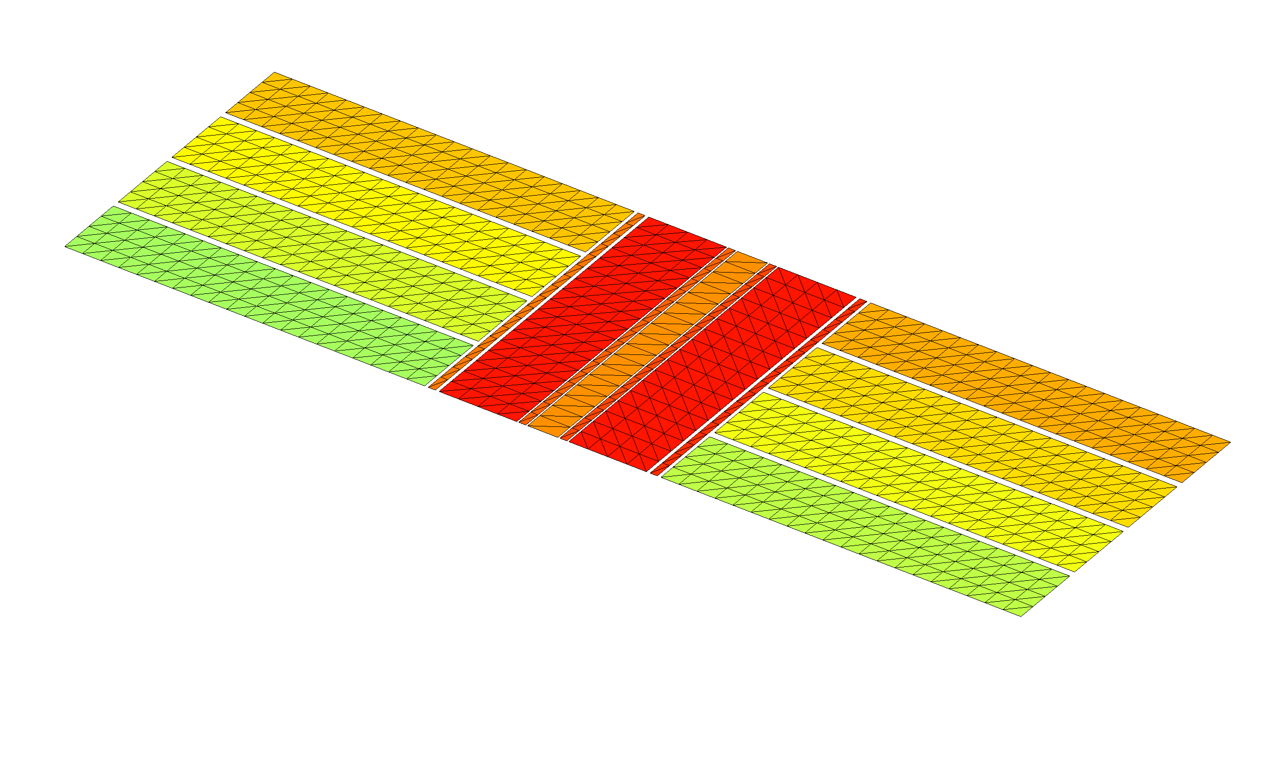
Visually confirming the geometry description

Before proceeding, we should certainly pause to check that the geometry defined by the improved geometry file does indeed look like what we want. We do this by running the scuff-analyze utility with the --WriteGMSHFiles command-line option:

% scuff-analyze --geometry Trap_4_Improved.scuffgeo --WriteGMSHFiles

This produces a file named Trap_4_Improved.pp, which we open in gmsh for visual confirmation:

% gmsh Trap_4_Improved.pp

Phase 1 calculation: Computing fields of individual conductors

The first phase of our calculation will be to determine the electrostatic field configurations produced by holding each of the individual electrodes at a potential of 1 V with all other electrodes grounded. This will yield 8 distinct field configurations, which we can sample at an arbitrary set of evaluation points or visualize in graphical form; the electrostatic field obtained by driving all conductors with arbitrary specified voltages will be a weighted linear combination of these 8 configurations, so we can use the elemental fields to optimize a set of electrode voltages to yield a given field profile (phase 2, below).

Running multiple calculations at once: The excitation file

One obvious way to do this calculation would be to run scuff-static 8 times, each time using the --PotFile command-line option to define a different set of conductor potentials.

However, such an approach would be inefficient given the structure of the boundary-element method (BEM) implemented by scuff-static. In BEM solvers, almost all of the computational cost goes into assembling and factorizing the system matrix, which knows only about the geometry itself and is independent of any excitation that may furnish the stimulus in an electrostatics problem (such as externally-sourced fields or sets of prescribed conductor potentials). Thus, in cases where we wish to consider the response of a geometry to multiple stimuli, it is efficient to do the calculations all at once; having paid the cost of forming and factorizing the system matrix, we can solve electrostatics problems for any number of distinct stimuli essentially for free.

To allow this efficiency to be exploited in command-line calculations, scuff-static allows users to specify an excitation file describing one or more stimuli to be applied to the geometry sequentially. For the purposes of our first calculation, the excitation file will specify 8 separate stimuli, each consisting of a choice of one conductor to be held at a potential of 1.0 V (by default, any conductors not specified are maintained at 0 V). This file is called Phase1.Excitations:

EXCITATION UpperDC1
    UpperDC1 1.0
ENDEXCITATION

EXCITATION LowerDC1
    LowerDC1 1.0
ENDEXCITATION

EXCITATION UpperDC2
    UpperDC2 1.0
ENDEXCITATION

EXCITATION LowerDC2
    LowerDC2 1.0
ENDEXCITATION

EXCITATION UpperDC3
    UpperDC3 1.0
ENDEXCITATION

EXCITATION LowerDC3
    LowerDC3 1.0
ENDEXCITATION

EXCITATION UpperDC4
    UpperDC4 1.0
ENDEXCITATION

EXCITATION LowerDC4
    LowerDC4 1.0
ENDEXCITATION

This file is passed to scuff-em via the --ExcitationFile command-line option. Notice that each EXCITATION is labeled by an arbitrary user-defined tag, which will be used to identify the output produced under that excitation.

Speaking of outputs, we will want to tell scuff-static what we'd like it to compute for each excitation. In this case I'll ask for two types of output:

numerical values of the electrostatic potential and field at a set of evaluation points I choose; I will choose a line of points lying slightly above the structure and running down the center conductor. I put the coordinates of these points into a text file called MyEPFile and say --EPFile MyEPFile on the scuff-static command line.
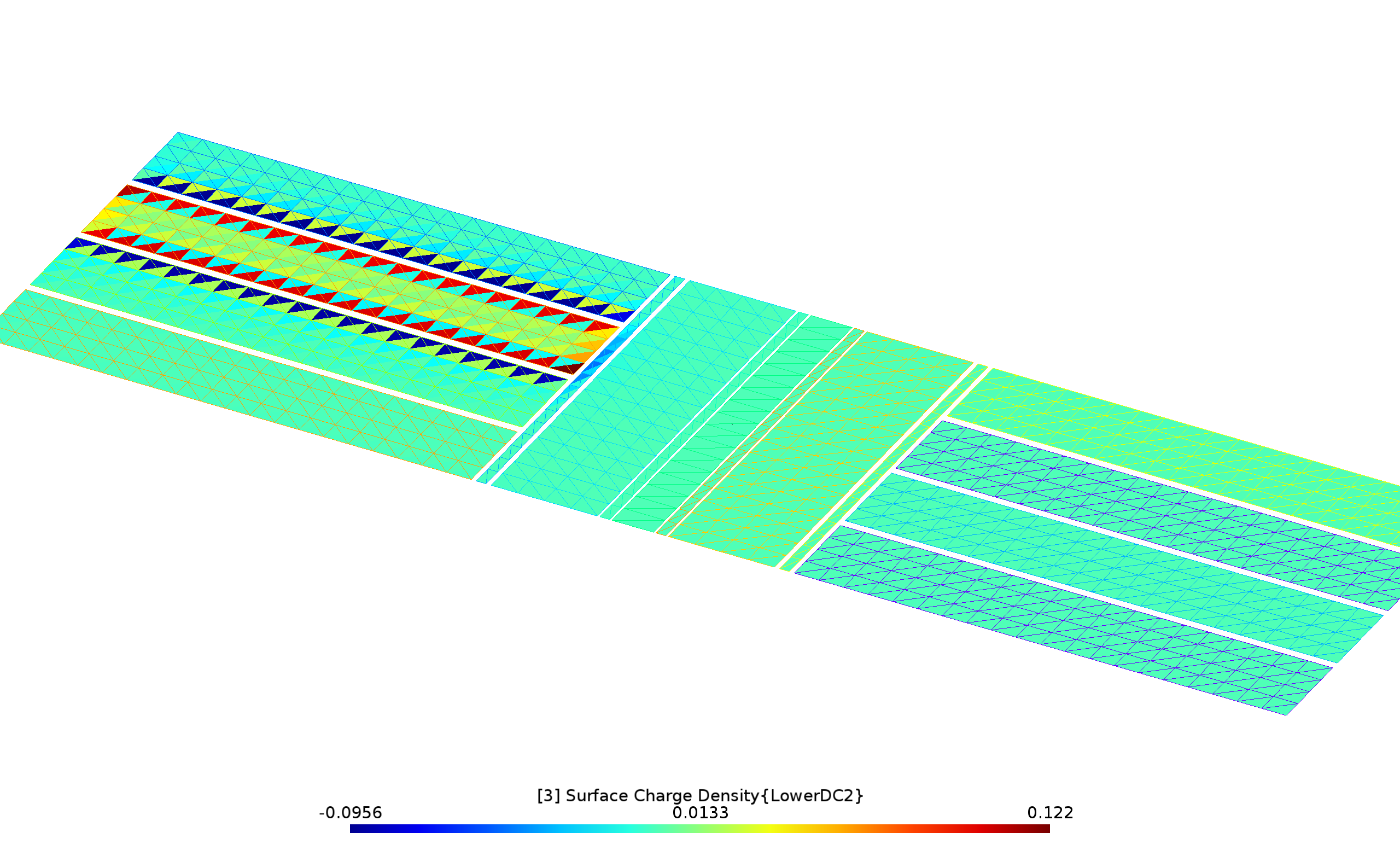
graphical visualization files showing the distribution of surface charge induced on the geometry by each exciting stimulus. (See below for a different type of graphical visualization output.) To request this I use the --PlotFile option to specify the visualization output file name (here I call it MyPlotFile.pp).

Here's a script (Phase1.RunScript) that runs the phase-1 calculation:

#!/bin/bash

ARGS=""
ARGS="${ARGS} --geometry Trap_4_Improved.scuffgeo"
ARGS="${ARGS} --ExcitationFile Phase1.Excitations"
ARGS="${ARGS} --EPFile MyEPFile"
ARGS="${ARGS} --PlotFile MyPlotFile.pp"
scuff-static ${ARGS}

This script takes about 3 seconds to run on my laptop. When it's finished, you have two new output files:

Trap_4_Improved.MyEPFile.out is a text data file reporting values of the electrostatic potential and field components at each evaluation point in MyEPFile for each excitation.
MyPlotFile.pp is a gmsh visualization file plotting the induced charge density for each of the 8 excitations. For example, here's what it looks like when the electrode named LowerDC2 is driven:

Phase 2 calculation: External sources and field visualization

Having determined the fields produced by each electrode in isolation, in practice we would now presumably do some sort of design calculation to identify the optimal voltages at which to drive each electrode for our desired application. As a follow-up calculation, we'll now do a run in which (a) each conductor is set to a nonzero voltage, (b) additional external field sources are present, (c) we wish to visualize the electrostatic fields over a region of space.

Items (a) and (b) are handled by writing an excitation file (Phase2.Excitations) that specifies, in addition to prescribed conductor potentials, several external field sources that are also present in the geometry: a point monopole, a point dipole, a constant electric field, and an arbitrary user-specified function. (Needless to say, this contrived assortment of sources is intended primarily to illustrate the types of external-field sources that may be specified in excitation files).

EXCITATION KitchenSink

# conductor potentials 

    UpperDC1   0.5
    LowerDC1  -0.7
    UpperDC2  -0.3
    LowerDC2   0.5
    UpperDC3   0.2
    LowerDC3  -0.4
    UpperDC4  -0.6
    LowerDC4   1.0

# point charge at X=(-400,1000,250) with charge -300
    monopole -400.0 1000.0 250.0   -300

# z-directed point dipole at X=(-300,-1000,-400)
    dipole  -300.0 -1000.0 -400.0  0.0 0.0 10000.0

# small constant background field in Z-direction
    constant_field 0 0 1.0e-4

# arbitrary user-specified function of x, y, z, r, Rho, Theta, Phi
        phi 1.0e-8*Rho*Rho*cos(2.0*Phi)

ENDEXCITATION

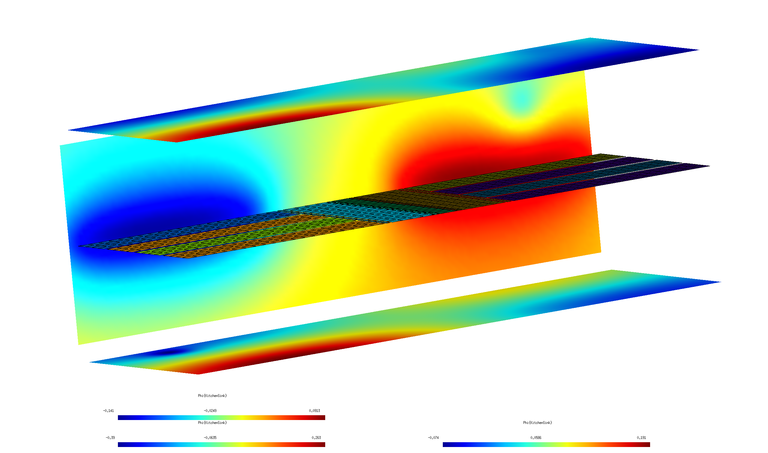
Item (c) is handled by using gmsh to define a field-visualization mesh---in essence, a screen on which we want an image of the electrostatic field configuration, although it need not be planar---together with a set of geometrical transformations specifying how the screen is to be replicated throughout space to yield quasi-3D visual information on the field configuration. In this case, the mesh is described by the simple gmsh geometry file Screen.geo, which we turn into Screen.msh by running gmsh -2 Screen.geo. Then, the transformation file Screen.trans specifies three geometrical transformations in which the screen is rotated and displaced to define the three walls of the diorama shown in the figure below.

The script that runs the calculation is Phase2.RunScript:

#!/bin/bash

ARGS=""
ARGS="${ARGS} --geometry Trap_4_Improved.scuffgeo"
ARGS="${ARGS} --ExcitationFile Phase2.Excitations"
ARGS="${ARGS} --FVMesh Screen.msh"
ARGS="${ARGS} --FVMeshTransFile Screen.trans"
scuff-static ${ARGS}

This produces several files with extension .pp; we open them all simultaneously in gmsh together with the original geometry mesh to get some graphical insight into the spatial variation of the fields in our problem.

 % gmsh Trap_4*.pp Trap_4.msh

Click the image below for higher resolution: