Incident fields in scuff-em
For the classical scattering problems solved by scuff-scatter or by C++ or python codes using the scuff-em API, you will want to specify the incident fields that scatter from your geometry.
The default scuff-em distribution offers three built-in types of incident fields:
If you only need to run scattering calculations with a single type of incident field, you can just specify that field on the command line, as described in the sections below. If you want to run scattering calculations with multiple types of incident field (for example, perhaps at each frequency you want to consider two different plane-wave polarizations, or three different point-source locations) you will want to write an incident-field file describing an entire list of incident fields.
It is also easy to define your own custom incident fields for use in API programs.
Built-in types of incident field
Plane waves
scuff-scatter command-line syntax:
--pwDirection nx ny nz
--pwPolarization Ex Ey Ez
C++ code:
  double  nHat[3] = {nx, ny, nz};
  cdouble E0[3]   = {Ex, Ey, Ez};
  PlaneWave *PW=new PlaneWave(E0, nHat);
Selects the incident field to be a plane wave, with propagation vector n=(nx,ny,nz) and E-field polarization vector E=(Ex,Ey,Ez).
More specifically, the fields of a plane wave are
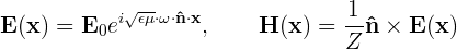
where the components of the vectors
and
are what you specify with the --pwDirection and
--pwPolarization options to scuff-scatter. (The frequency
is specified elsewhere, for example using
command-line options like --omega. The
quantities and are the material properties of
the exterior medium at this frequency, which are determined by
the material property designation you give the external medium
in the .scuffgeo file; the wave impedance of the medium is
in vacuum.)
The values specified for --pwPolarization may be
complex numbers.
As an example, the scuff-scatter command-line options
--pwDirection 0 0 1 --pwPolarization 0.7071 0.7071i 0.0
will specify an incident field consisting of a circularly polarized plane wave traveling in the positive z direction.
Gaussian beams
scuff-scatter command-line syntax:
--gbCenter Cx Cy Cz
--gbDirection nx ny nz
--gbPolarization Ex Ey Ez
--gbWaist W
C++ code:
  double X0[3]={Cx, Cy, Cz};     /* beam center point */
  double KProp[3]={nx, ny, nz};  /* beam propagation vector */
  cdouble E0[3]={Ex, Ey, Ez};    /* complex field-strength vector */
  double W0=W;                   /* beam waist */
  GaussianBeam *GB=new GaussianBeam(X0, KProp, E0, W0);
Selects the incident field to be a focused Gaussian beam,
traveling in the direction defined by the unit vector
n=(nx,ny,nz), with E-field polarization
vector E=(Ex,Ey,Ez), beam center point with cartesian
coordinates C=(Cx,Cy,Cz), and beam waist W.
The values specified for --gbPolarization may be
complex numbers.
The scuff-em implementation of the field of a Gaussian laser beam was contributed by Johannes Feist and follows this paper:
- Sheppard and Saghafi, "Electromagnetic Gaussian Beams Beyond the Paraxial Approximation," Journal of the Optical Society of America A 16 1381 (1999), http://dx.doi.org/10.1364/JOSAA.16.001381.
Point sources
scuff-scatter command-line syntax:
--psStrength Px Py Pz
--psLocation xx yy zz
C++ code:
  double  X0[3] = {xx, yy, zz};
  cdouble P0[3] = {Px, Py, Pz};
  PointSource *PS=new PointSource(X0, P0);
Selects the incident field to be the field of a pointlike
electric dipole radiator with dipole moment P=(Px,Py,Pz)
and located at cartesian coordinates (xx,yy,zz).
More specifically, the fields of a point source are given by
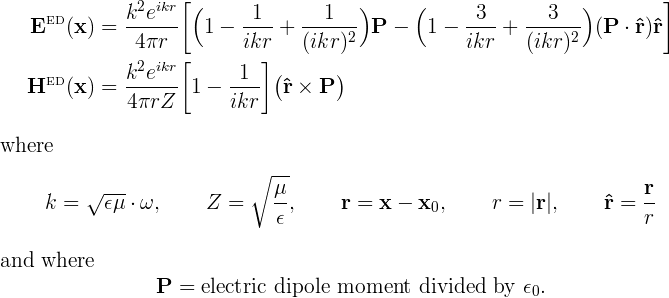
The values specified for --psStrength may be
complex numbers.
You may define the incident field to be a superposition of
the fields of multiple point sources by specifying these
options more than once. (The nth occurrence of --psStrength
will be paired with the nth occurrence of --psLocation.)
In API codes (but not in scuff-scatter) it is also possible to a define a magnetic point source as follows:
PointSource *PS=new PointSource(X0, P0);
Specifying an entire list of incident fields
A feature of the surface-integral-equation solver implemented by scuff-em is that, once the computational work needed to solve a single scattering problem (for a given geometry at given frequency irradiated by a single incident field) has been done, there is relatively little computational cost required to solve additional problems (for the same geometry at the same frequency) with different incident fields. To exploit this feature, you may write an "incident-field file" (a simple text file) describing multiple types of incident field with which to irradiate your geometry.
Example of an incident-field file
Here's an example of an incident-field file describing 9
different incident fields. If you specify this file
using the --IFFile command-line option to
scuff-scatter,
then every calculation you request (scattered fields,
power/force/torque, visualization, etc.) will be
done 7 times at each frequency, once for each field.
EX    PW    0  0  1       1          0          0
EY    PW    0  0  1       0          1          0
LC    PW    0  0  1       0.7071     0.7071i    0
RC    PW    0  0  1       0.7071    -0.7071i    0

PS1   PS    1.1 2.2 3.3   0.4+0.5i   0.7        -0.8
PS2   MPS   1.1 2.2 3.3   0.4+0.5i   0.7        -0.8

GB    GB    0.0 0.0 0.0   0.0 0.0 1.0    1.0 0.0 0.0    0.5

COMPOUND1
  PW    0   0  1      1        0        0
  PS    1.1 2.2 3.3   0.4+0.5i 0.7      -0.8
END

COMPOUND2
  PW    0   0  1      0        1        0
  PS    1.1 2.2 3.3   0.4+0.5i 0.7      -0.8
END
Here's how to understand the 9 incident fields described by this file.
-
The first several lines define various types of incident fields in which there is only a single field source. For this type of incident field, the first word on the line is an arbitrary user-specified label (such as
EXorPS1) that will be used to identify data corresponding to this incident field in output files. The second word on the line is one of the four keywordsPW|PS|MPS|GB. The remainder of the line consists of numerical parameters:-
For plane waves (keyword
PW) there are 6 numerical parameters:nx ny nz Ex Ey Ez. In the example above,EXandEYare linearly-polarized plane waves, whileLCandRCare left- and right-circularly polarized waves. -
For electric-dipole point sources (keyword
PS) there are 6 numerical parameters:xx yy zz Px Py Pz. -
For magnetic-dipole point sources (keyword
MPS) there are 6 numerical parameters:xx yy zz Mx My Mz. -
For gaussian beams (keyword
GB) there are 10 numerical parameters:Cx Cy Cz nx ny nz Ex Ey Ez W.
-
-
The final two sections of the file describe compound fields---that is, incident fields produced by more than one source acting simultaneously. These types of fields are described by putting their label (here
COMPOUND1orCOMPOUND2) on line by itself, then specifying as manyPW|PS|MPS|GBlines as you like, and finally closing the compound-field definition with theENDkeyword. For example, the field we labeledCOMPOUND1consists of a planewave acting simultaneously with the field of a point source.
Using incident fields in API programs
Please see here for further details and examples of how incident fields are manipulated in API codes, including an example of how to create your own custom-designed incident field.