

Casimir forces between infinitely extended silicon beams (1D periodicity)

In this example, we exploit scuff-em's support for 1D periodic geometries to compute the equilibrium Casimir force per unit length between infinitely extended silicon beams of rounded rectangular cross section. The files for this example may be found in the share/scuff-em/examples/SiliconBeams subdirectory of your scuff-em installation.

gmsh geometry file for unit-cell geometry

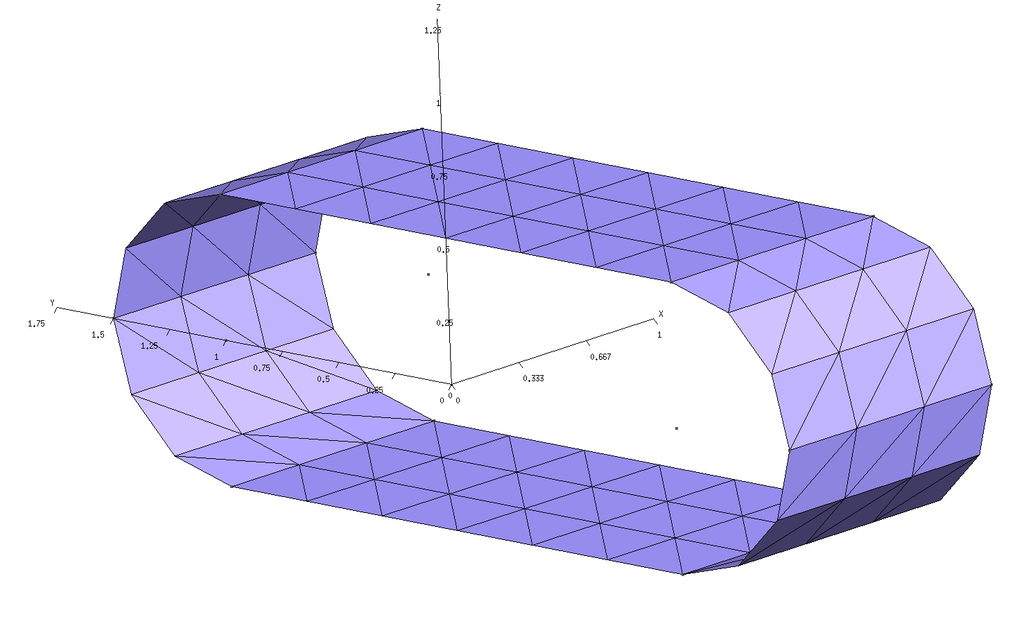
The gmsh geometry file RoundedBeamUnitCell.geo describes the portion of the surface of a single beam that lies within the unit cell, i.e. the cell that is infinitely periodically replicated to yield the full geometry. To produce a discretized surface-mesh representation of this geometry, we run it through gmsh:

% gmsh -2 RoundedBeamUnitCell.geo

This produces the file RoundedBeamUnitCell.msh, which I rename to RoundedBeamUnitCell_192.msh because 192 is the number of interior edges (this information may be found, for example, by running scuff-analyze --mesh RoundedBeamUnitCell.msh). You can open the .msh file in gmsh to visualize the unit-cell mesh:

% gmsh RoundedBeamUnitCell_192.msh

Unit cell mesh picture

Note the following:

For 1D periodic geometries in scuff-em, the direction of infinite extent must be the x direction.
Only the sidewall of the cylinder is meshed; the endcaps must not be meshed.
For surfaces that straddle the unit-cell boundaries (as is the case here), each triangle edge that lies on the unit-cell boundary must have an identical image edge on the opposite side of the unit cell. An easy way to achieve this is to use extrusions in gmsh, as in the .geo file above.
In this case the unit cell is 1 $\mu$ m long. (More generally, the unit cell could have any length you like.)

scuff-em geometry file

The scuff-em geometry file describing our two infinite-length silicon beams is SiliconBeams_192.scuffgeo. This specifies a geometry consisting of two identical silicon beams, of infinite extent in the x direction, separated by a distance of 2 $\mu$ m in the $z$ direction. The infinite beams consist of the finite-length unit-cell geometry, periodically replicated infinitely many times. (The length of the lattice vector specified by the LATTICE statement should agree with the length of the unit cell as defined in the gmsh geometry file.)

LATTICE
    VECTOR 1.0 0.0
ENDLATTICE

MATERIAL SILICON
    epsf = 1.035;      # \epsilon_infinity
    eps0 = 11.87;      # \epsilon_0 
    wp = 6.6e15;       # \plasmon frequency
    Eps(w) = epsf + (eps0-epsf)/(1-(w/wp)^2);
ENDMATERIAL

OBJECT Beam1
    MESHFILE RoundedBeamUnitCell_192.msh
    MATERIAL Silicon
ENDOBJECT

OBJECT Beam2
    MESHFILE RoundedBeamUnitCell_192.msh
    MATERIAL Silicon
    DISPLACED 0 0 2
ENDOBJECT

We can use scuff-analyze to visualize the geometry described by this .scuffgeo file:

% scuff-analyze --geometry SiliconBeams_192.scuffgeo --WriteGMSHFiles --Neighbors 2

[The option --Neighbors 2 requests that, in addition to the unit-cell geometry, the first 2 periodic images of the unit cell in both the positive and negative directions (for a total of 5 copies of the unit cell) be plotted as well. This helps to convey a slightly better sense of the actual infinite-length structure being simulated.] This produces the file SiliconBeams_192.pp, which you can view in gmsh:

% gmsh SiliconBeams_192.pp

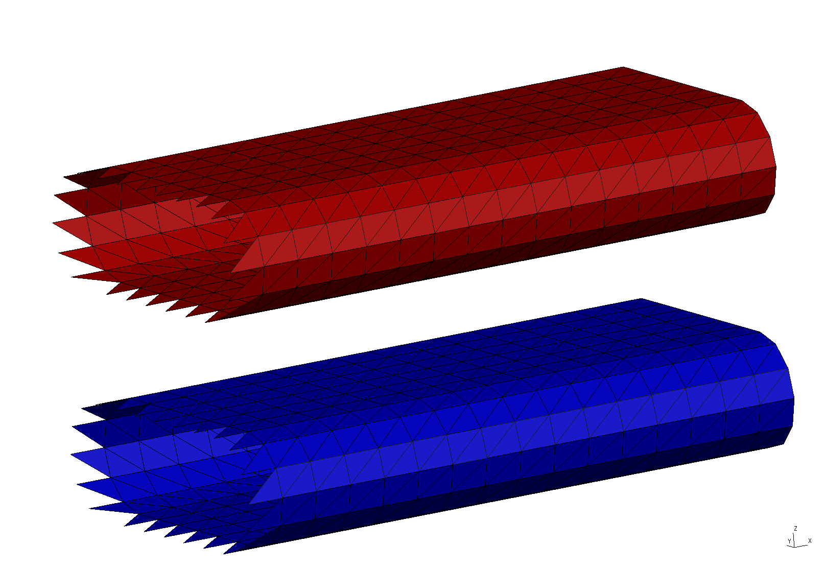
Geometry visualization file picture

Note that the visualization file produced by scuff-analyze includes extra triangles (visible at the left end of the structure) that are not present in the unit-cell geometry. These are called straddlers, and they are added automatically by scuff-em to account for surface currents that flow across the unit-cell boundaries in periodic geometries.

scuff-em transformation file

In Casimir problems we typically want to compute forces (or torques, or energies) at multiple values of the surface--surface separation. This is done by writing a transformation file. In this case we'll request the Casimir force between the beams for 9 distinct values of the surface-surface separation ranging between 1-5 $\mu$ m. The file that specifies this is called Beams.trans:

TRANS 1.00 OBJECT Beam2 DISP 0 0 0.00
TRANS 1.50 OBJECT Beam2 DISP 0 0 0.50
TRANS 2.00 OBJECT Beam2 DISP 0 0 1.00
TRANS 2.50 OBJECT Beam2 DISP 0 0 1.50
TRANS 3.00 OBJECT Beam2 DISP 0 0 2.00
TRANS 3.50 OBJECT Beam2 DISP 0 0 2.50
TRANS 4.00 OBJECT Beam2 DISP 0 0 3.00
TRANS 4.50 OBJECT Beam2 DISP 0 0 3.50
TRANS 5.00 OBJECT Beam2 DISP 0 0 4.00

For full details on scuff-em transformation files, see this reference page. For the time being, note the following:

The text TRANS 4.00 specifies the string 4.00 as the name of this transformation. This is the string that will be written to output files to identify the Casimir quantities corresponding to each geometrical transformation. This can be any string not including spaces (in particular, it need not be a number), but it's usually convenient to label transformations by numbers so that we can subsequently plot e.g. force vs. distance.
The text OBJECT Beam2 DISP 0 0 3.00 specifies that, in this particular geometrical transformation, the object labeled Beam2 in the .scuffgeo file is to be displaced 3 $\mu$ m in the z direction.
Why do we assign the label 4.00 to a transformation in which the displacement is 3 $\mu$ m? Because transformations are relative to the configuration described in the .scuffgeo file, and in the .scuffgeo file discussed above the second beam is already displaced a distance of 2 $\mu$ m from the first beam, which means the default surface-surface separation is 1 $\mu$ m. Applying an addition 3 $\mu$ m displacement then yields a surface-surface separation of 4 $\mu$ m.

You can use scuff-analyze to obtain a visualization of what your geometry looks like under each transformation:

% scuff-analyze --geometry SiliconBeams_192.scuffgeo --TransFile Beams.trans

This produces a file named SiliconBeams_192.transformed.pp, which you can open in gmsh to confirm that the transformations you got are the ones you wanted.

A first trial run of scuff-cas3d at a single frequency

To compute the full Casimir force per unit length between the beams (call this quantity $\mathcal F$ ), scuff-cas3d numerically evaluates an integral over both imaginary frequencies $\xi$ and Bloch wavenumbers $k$ : $\mathcal F = \int_0^\infty d\xi \underbrace{\left [ \frac{1}{V_{\scriptsize{BZ}}} \int_{V_{\scriptsize{BZ}}} f(\xi, k) dk \, \right] }_{\equiv F(\xi)}$ where the $k$ integral is over the Brillouin zone (BZ) and $V_{\scriptsize{BZ}}$ is the one-dimensional volume of the BZ. For a 1D periodic geometry, the Brillouin zone is the 1D interval $0\le k \le \frac{2\pi}{L}$ , and its one-dimensional volume (its length) is $\frac{2\pi}{L}$ , where $L=1\, \mu$ m is the length of the real-space unit cell. , Because the full calculation can be somewhat time-consuming, it's often useful to run a quick single-frequency calculation just to make sure things are making sense before launching the full run. We do this by specifying the --Xi command-line option to scuff-cas3d, which requests a calculation of just the quantity $F(\xi)$ in the above equation at a single imaginary frequency $\xi$ . (Note that, for our 1D periodic geometry, this single-frequency calculation still entails a wavenumber integration over the 1D Brillouin zone.)

 % scuff-cas3d --geometry SiliconBeams_192.scuffgeo --TransFile Beams.trans --zforce --xi 0.7

This produces (among other files) files called SiliconBeams_192.byXi and SiliconBeams_192.byXikBloch. The former file reports values of the quantity $F(\xi)$ , at the requested value of $\xi$ , for each of the transformations in the .trans file. The latter file gives more granular information: it reports values of the quantity $f(\xi,k)$ at the requested value of $\xi$ and at each $k$ point sampled by the built-in numerical integrator.

The file SiliconBeams_192.byXi looks like this:

# scuff-cas3D run on superhr1 at 06/07/15::01:01:38
# data file columns: 
#1: transform tag
#2: imaginary angular frequency
#3: z-force Xi integrand
#4: z-force error due to numerical Brillouin-zone integration 
1.00 7.000000e-01 1.53365587e-02 1.10343992e-05
1.50 7.000000e-01 3.27174955e-03 6.54894735e-06
...
5.00 7.000000e-01 2.84878401e-06 4.63609357e-08

As the file header says, the first column here is the transform tag (the surface--surface separation), the second column is the imaginary angular frequency in units of $\xi_0=3\cdot 10^{14}$ rad/sec, and the third column is the Casimir force per unit length per unit frequency (in units of $\hbar c/(\omega_0 L_0^3)=31.6 (\text{fN/micron})/\omega_0$ ) where $L_0=1\mu\text{m}$ and where $\text{fN}$ =femtoNewtons.

The full run

Now just launch the full run:

 % scuff-cas3d --geometry SiliconBeams_192.scuffgeo --TransFile Beams.trans --zforce

(This is the same command line as before, just without the --Xi option.)

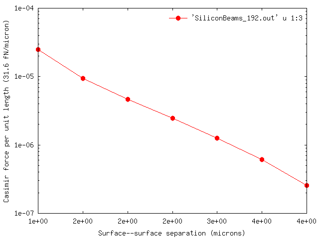
After some computation, this produces the output file SiliconBeams_192.out. You can plot the force (per unit length) versus surface--surface separation using e.g. gnuplot:

% gnuplot
gnuplot> set xlabel 'Surface--surface separation (microns)'
gnuplot> set ylabel 'Casimir force per unit length (31.6 fN/micron)'
gnuplot> set logscale y
gnuplot> plot 'SiliconBeams_192.out' u 1:3 w lp pt 7 ps 1.5

SiliconBeamData